Audio Generative Modeling in Latent Space

中文 · English

Contents

• 0. Introduction
• 1. What Makes Audio Special & Mel-spectrogram as an Early Latent
  • 1.1 Where audio and images differ
  • 1.2 Mel-spectrogram: the latent you’ve been using all along
• 2. The Discrete Direction: Audio as Language
  • 2.1 From VQ-VAE to SoundStream / EnCodec / DAC
  • 2.2 The popularity of RVQ: why most audio codecs choose residual quantization
  • 2.3 AudioLM’s semantic / acoustic paradigm
  • 2.4 Common patterns for downstream modeling
  • 2.5 The “modelability” toolbox of the discrete direction
• 3. The Continuous Direction: Audio as Latents
  • 3.1 First phase: adapting the vision template
  • 3.2 The latent’s semantic turn: meeting up with the discrete direction
  • 3.3 The “modelability” toolbox of the continuous direction
  • 3.4 Streaming: from the ceiling of NAR to continuous autoregression
  • 3.5 One piece of the puzzle still missing: streaming modeling of high-dimensional semantic latents
• 4. Synthesis: the two directions are converging, the real controversy lies elsewhere
  • 4.1 Discrete and continuous are converging on the same set of goals
  • 4.2 What will the unified interface be — a deeper RVQ, or lighter continuous features?
  • 4.3 Audio’s fixed-grid constraint is more severe than vision’s
  • 4.4 Adding streaming to Sander’s rate-distortion-modelability triangle
• 5. Closing: open problems
  • Will audio converge to a single unified latent?
  • End-to-end is harder in audio than in vision
  • The place of the audio latent in the multimodal era
  • Will the audio encoder / codec simply disappear?

0. Introduction

In April 2025, Sander Dieleman published a long-form post, Generative modelling in latent space¹. The post gives a useful way to think about latent representations in image generation: a good latent is not only about reconstruction quality, but also about rate, distortion, and modelability.

Audio generation faces a similar question, but the answer is less settled. Current systems roughly follow two directions. One direction represents audio as discrete codec tokens and models them with language models. The other represents audio as continuous latents and models them with diffusion or flow matching. These two directions are often presented as competing paradigms, but I think they are gradually moving toward the same set of goals.

This post discusses that convergence from the perspective of audio generation. The key question is not simply whether the latent should be discrete or continuous. The more important question is: what kind of representation is easy to model while still preserving the information needed for high-quality audio generation?

Audio makes this question harder than vision in two ways:

1. The fixed-grid constraint. Audio representations must balance frame rate, per-frame capacity, and sequence length. A low frame rate shortens the sequence but increases the burden on each frame; a high frame rate improves reconstruction but makes downstream modeling harder.
2. Streaming. For real-time speech interaction, the representation must be causal, compact, and low-latency. This turns streaming from an engineering preference into a hard constraint.

The rest of the post is organized as follows:

• §1 discusses why audio is different from images, and why mel-spectrograms can be viewed as an early handcrafted latent representation.
• §2 reviews the discrete-token direction: SoundStream, EnCodec, DAC, RVQ, AudioLM-style semantic/acoustic tokenization, and downstream LM modeling patterns.
• §3 reviews the continuous-latent direction: waveform/mel diffusion, latent diffusion, flow matching, and semantic continuous latents.
• §4 argues that the two directions are converging, and that the real design tension lies in frame rate, capacity, modelability, and streaming.
• §5 closes with several open questions about unified audio latents, end-to-end training, multimodal models, and whether the codec will remain an independent module.

The intended reader is an audio researcher or engineer. Familiarity with Sander’s post is helpful, but not required; I will briefly introduce the relevant concepts when they appear.

1. What Makes Audio Special & Mel-spectrogram as an Early Latent

It’s worth taking a step back here to ask a plain question: why did audio generation evolve into two directions: discrete and continuous? Image generation faces similar design choices too, so why is the divergence between these two directions sharper and harder to stitch back together in audio?

The answer has two layers. One is the physical properties of the audio signal itself — this determines the baseline constraints of all latent design. The other is that the mel-spectrogram, a handcrafted latent, occupied a central role in audio generation for the past decade, and its influence persists in codec design intuitions to this day. This section lays out these two things, setting up the later argument that “the two directions are converging.”

1.1 Where audio and images differ

The differences between audio and images in generative-model design are often reduced to “different sampling rates” — but that’s just the surface. There are four real differences that shape representation design:

1. A long-context one-dimensional signal. Audio is a high-sample-rate, long-unrolling one-dimensional sequence: 16 kHz speech is 16000 samples per second, 44.1 kHz music is 44100 per second. Compared with a 256×256 image’s total of 65536 pixels, the total sample count per second is actually about the same — the key difference isn’t quantity, it’s structure. An image’s 2D spatial grid can be compressed into a short 2D latent grid and processed in parallel; but once audio extends to tens of seconds or minutes, the number of time steps grows linearly and it quickly becomes a long-context modeling problem. So an audio latent must be aggressively downsampled along the time dimension (from 16/44 kHz down to the 25/50/75 Hz range, a ratio starting at 320×), otherwise the downstream LM / diffusion simply can’t ingest it.

2. The paradox of phase. The human ear is generally not sensitive to absolute phase — a change in the starting phase of a single sine wave, or a polarity flip of an entire clip, won’t noticeably change how it sounds. But the ear is very sensitive to structural distortion caused by phase errors — periodic or discontinuous phase deviations break the coherence between harmonics, producing a mechanical, metallic, or buzzing artifact; phase errors in transient regions change the local temporal structure of the waveform, blunting onsets and reducing punch. So in audio generation, phase itself need not be matched point-by-point largely, but the phase structure must remain natural and consistent.

This asymmetry deeply influences codec design. The mel-spectrogram directly discards phase (magnitude only), passing the job of recovering phase off to the vocoder. The training objectives of neural codecs implicitly acknowledge this too — EnCodec / DAC’s multi-scale STFT discriminator ingests the complex STFT (with phase), but adversarial training only requires it to “look real,” not to be sample-level strictly aligned; mel L1 is again largely magnitude-only; so the overall optimization pressure puts only a weak constraint on “point-by-point alignment of waveform phase to the reference,” defaulting to “sample alignment is the decoder’s private business,” filled in by the inductive bias the decoder learns.

3. The anisotropy of perception. In vision, a learned perceptual similarity metric like LPIPS offers a relatively stable, differentiable approximation of perceptual distance — and when combined with reconstruction / adversarial / diffusion objectives, it often improves the perceptual quality of generation. Audio lacks an equally recognized, general, training-stable counterpart. The traditional tools of psychoacoustics (mel filterbank, Bark filterbank, auditory masking) are themselves differentiable; mel L1 is a loss used daily in codec training — but they are handcrafted local auditory approximations, hard to fully cover the more complex perceptual dimensions of timbre naturalness, transient clarity, and phase-structure consistency. On the evaluation side, PESQ / STOI are usually unsuitable as training losses; learned MOS predictors like UTMOS can serve as a loss or reward, but optimizing them directly tends to introduce metric bias and may not generalize to all codec designs. The result is that codec training can only stack a group of indirect objectives — multi-scale STFT, mel loss, waveform loss, multi-period discriminator — approaching the true perceptual experience from different local viewpoints, rather than constraining generation directly with a single LPIPS-style loss the way vision can.

4. Texture and structure: the audio version of stuff vs things. Sander’s original article has a nice framing: image content divides into texture (stuff) and structure (things). The texture of grass is high-entropy, but the eye cannot distinguish different realizations of the same texture — what we perceive is the uncountable category “grass,” not each individual blade. Original and reconstruction look identical side by side; only by overlaying them and toggling back and forth do you expose that the texture regions actually differ a lot. Whereas for structure like a dog’s eye, the same magnitude of difference is immediately seen. So a good latent should abstract away texture and preserve structure — recording only “there is grass here,” not the position of every blade. This lets the autoencoder discard a huge texture modality, and lets the generative model on the latent only model the “presence or absence” of texture, without having to memorize all of texture’s entropy.

Audio has a fully corresponding phenomenon, and psychoacoustics gave it a name long ago — sound texture. McDermott & Simoncelli’s² classic work showed that sounds like rain, applause, the crackle of fire, and insect chirping are perceived by the ear through time-averaged statistics, not through the concrete waveform realization — two stretches of rain with different realizations but identical statistics sound like the very same rain. The counterpart in speech is more familiar: the essence of unvoiced consonants /s/ /f/ is noise shaped by a spectral envelope, and under the same envelope, swapping in a different noise realization leaves the perception mostly unchanged; reverberation tails are statistically perceived too — we hear “the room is big,” not each individual reflection. These are audio’s stuff. Audio’s things, on the other hand, are: the fundamental-frequency trajectory (slightly off and you hear it immediately), formants (which determine phoneme identity), transients (the attack of a piano, the burst of a plosive — smear them slightly in time and they’re ruined). The same magnitude of deviation, if it affects texture, is inaudible; if it affects structure, it’s a jarring artifact. Note this is closely related to the phase paradox in point 2: the phase of the noise component is pure texture (fully exchangeable), while the phase relationships between harmonics are structure (coherence must be preserved).

But there’s an important difference between audio and vision, and it’s one reason the audio latent is harder to build: vision’s texture and structure are partitioned in space, while audio’s are superimposed in time-frequency. In one image, grass occupies one region and the dog’s eye another, and the latent can allocate capacity by spatial position; whereas in audio, /s/ follows a vowel within tens of milliseconds, the reverb tail overlaps onto the next syllable, the noise wash of a cymbal and the bass line exist in the same frame at once. To “abstract texture and preserve structure,” vision can rely on spatial allocation, but audio must rely on some kind of component decomposition — harmonic vs noise, periodic vs aperiodic.

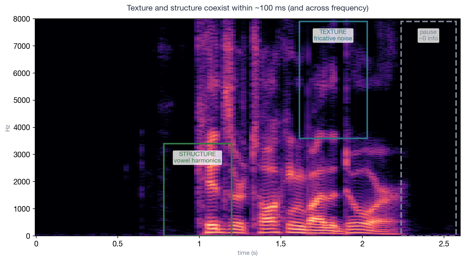
caption: “Within a single utterance, texture and structure sit less than a hundred milliseconds apart: the green box holds the harmonic striations of a vowel (structure — the fundamental-frequency trajectory, slightly off and you hear it immediately), the blue box holds the noise block of /s/ (texture — swap in a different noise realization and the perception is identical), and the dashed box holds a pause (almost zero information). In vision, grass and the dog’s eye each occupy a region; in audio these three things alternate along the same time axis and coexist in different frequency bands of the same frame — this is what ‘time-frequency superposition’ means, and it’s the direct cause of constant-frame-rate codecs wasting capacity.”

An important point is that classic audio coding was already doing this decades ago. LPC splits the excitation signal into “periodic pulse train vs noise”; vocoders like STRAIGHT / WORLD have dedicated aperiodicity parameters; AAC’s PNS (Perceptual Noise Substitution, 1997) simply encodes a noise-type band as a flag bit plus an energy value — and regenerates it with random noise at decode time. “Encode only the presence and statistics of texture, not its realization” — the latent design principle Sander described was already used by audio coding engineers in the ’90s as a bit-saving trick. This generation of neural codecs actually inherited the intuition, only it replaced explicit component decomposition with implicit adversarial training: the noise realization produced by a GAN-based decoder doesn’t align sample-by-sample with the original signal but is statistically equivalent — which is largely the perceptual-science root of the “DAC negative SI-SNR” phenomenon §2.1 will discuss, and the audio version of Sander’s “image-overlay experiment.”

These four differences jointly lead to one thing: audio cannot directly adopt vision’s latent framework; it must have its own design philosophy. All the divergences between the §2 discrete direction and the §3 continuous direction are responses to these four constraints. The texture/structure one will keep coming back: the success of the mel + vocoder paradigm (§1.2) is essentially a single texture abstraction, and the fact that texture segments need only statistics while structure segments need dense bits is the information-theoretic root of §4’s “fixed-grid constraint.”

1.2 Mel-spectrogram: the latent you’ve been using all along

The most influential “latent” in audio generation isn’t learned. The mel scale comes from psychoacoustics, and mel-based features became standard in speech processing decades ago. Today, one line of Python computes it:

mel = librosa.feature.melspectrogram(y=waveform, sr=22050, n_mels=80)

You get a [T, 80] matrix. And then you use it as a latent — upstream you generate it from text with Tacotron or FastSpeech, downstream you synthesize the waveform from it with HiFi-GAN³. This paradigm ran for five years, produced dozens of highly cited papers, and was still the default front-end of TTS papers as of 2022.

We didn’t call it an “audio VAE” or “audio learned latent.” It was just called “mel-spectrogram” — a 1980s engineering concept. But if you take the two-stage latent framing Sander laid out and apply it here, you’ll find a slightly uncomfortable truth: mel perfectly satisfies all the properties a “learned latent” should have, except it isn’t learned — it’s handcrafted.

Let’s go through it one by one.

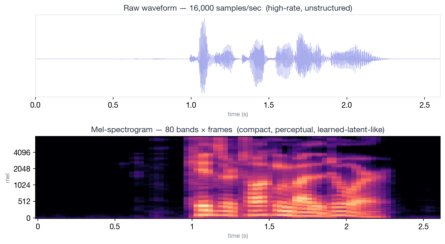
caption: “This is the ‘latent’ that TTS was actually modeling during the five years of 2017-2022 — it isn’t even learned, it’s computed by one line of Python. But it discards phase, compresses high frequencies, and mimics the human ear — everything a learned latent is supposed to do, it does.”

Lossy? Mel discards phase outright. An 80-dimensional magnitude vector cannot uniquely recover the STFT, let alone uniquely recover the waveform — so recovering audio from mel is essentially an ill-posed problem, requiring a vocoder (whether Griffin-Lim or HiFi-GAN) to “guess” a plausible phase. In the language of §1.1 point 4: what mel discards is largely audio’s largest source of texture entropy (the phase realization of the noise component), and what it preserves is largely structure (harmonic positions, formants, the energy contour) — mel is a handcrafted texture abstraction, and the vocoder’s job is to hallucinate a perceptually equivalent texture realization. This design of “discarding some dimensions and having the decoder fill them back in” is spiritually the same as VQGAN compressing a 256×256 image into a 16×16 latent — both assume the discarded part isn’t important and the decoder can fill it in from context.

Structured? Mel isn’t a flat vector, it’s a time-frequency 2D grid. Each time step corresponds to a frame (about 12.5 ms), each frequency bin to a band on the mel scale. VQGAN’s latent is also a 2D grid (spatial); mel is a 2D grid (time × frequency). Neither expects to compress “content” into a single fixed vector; instead each retains a low-resolution structured representation — a “signal thumbnail” that downstream can easily ingest.

Perceptually motivated? The mel scale wasn’t chosen arbitrarily by engineers; its origins aren’t even related to audio processing — in 1937, three experimental psychologists, Stevens, Volkmann, and Newman, ran a set of purely subjective experiments: they had listeners adjust pitch so that one tone sounded “exactly half as high” as another, and from this measured the nonlinear mapping between subjective pitch and physical frequency; the word “mel” was taken from melody⁴. Turning it into a speech feature would wait until Davis & Mermelstein’s MFCC in 1980⁵. In other words, mel is a byproduct of 1930s research into “how the human ear hears,” not something anyone designed to model audio. But largely because it faithfully compresses in auditory perceptual structure — the logarithmic frequency axis corresponding to the response of the cochlear basilar membrane (fine at low frequencies, coarse at high), critical bands corresponding to masking effects — using mel as a latent is equivalent to getting a human-ear “perceptual prior” for free. This is closely related to what VQGAN tries to learn with an LPIPS-style perceptual loss, except mel was assembled by hand from psychoacoustic common sense, decades in advance.

Good modelability? This point is the most practical. Mel frames have strong temporal correlation between them, friendly to both RNN and transformer; the dimensionality is 80, two orders of magnitude lower than 22050 Hz waveform. This is why in 2017 Tacotron chose the two-stage text-to-mel + vocoder — learning end-to-end text-to-waveform generation was too hard to model at the time, while text-to-mel lowered the modeling difficulty by an order of magnitude.

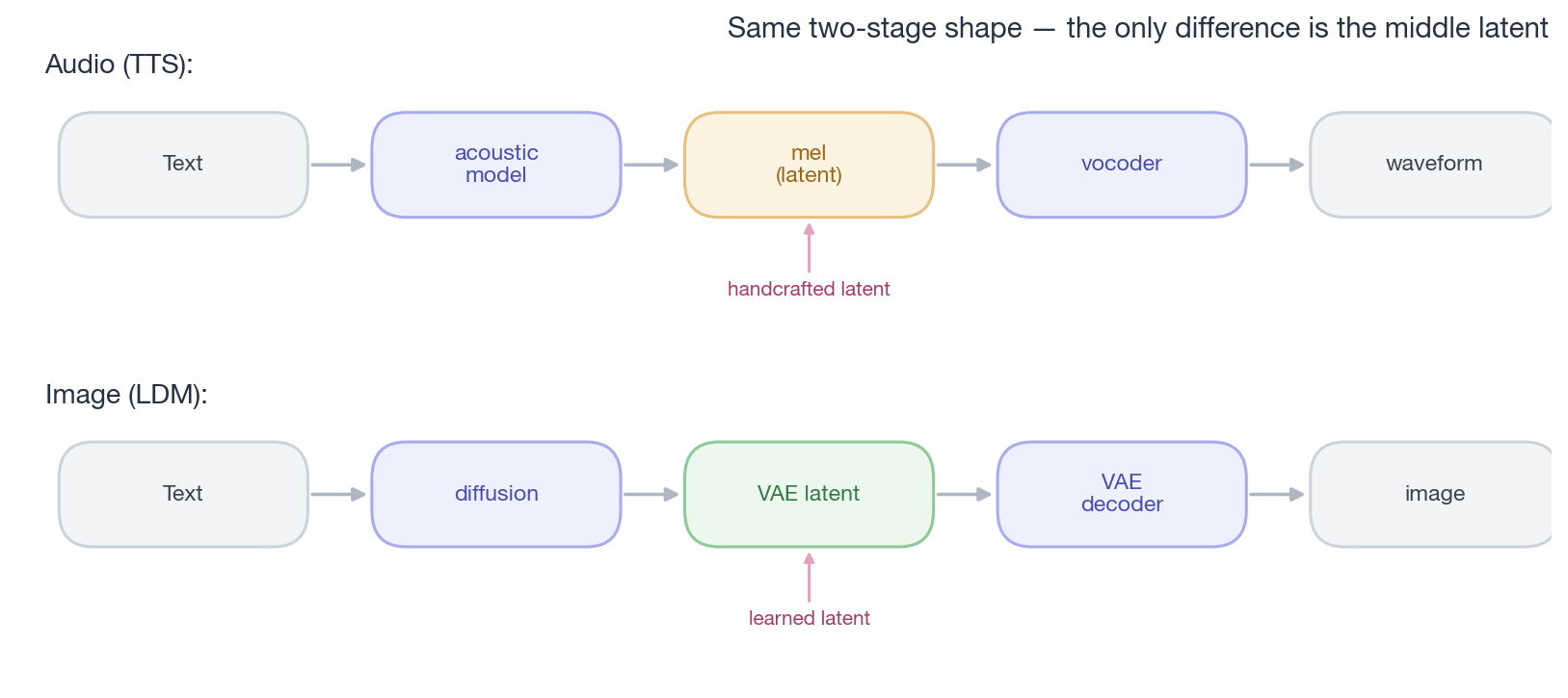
caption: “The two-stage paradigm in the two fields is structurally identical. The only difference is that audio’s middle latent layer is handcrafted while the image’s is learned. So the question isn’t ‘should audio go down the LDM road,’ but ‘when do we replace the handcrafted latent with a learned one.’”

This paradigm really ran very well. Tacotron 1/2⁶, FastSpeech 1/2, Glow-TTS, VITS — the entire golden age of TTS from 2017-2022 lived in this framework. Under single-speaker + enough data + a controlled scenario, the output was already good enough that people couldn’t tell over a short span that it was synthesized. If you pile all the TTS papers of those five years together, you’ll notice something interesting: everyone was improving the first stage (text-to-mel), but few people questioned why the second stage was mel. Mel had practically become the “physics of audio” that everyone accepted by default — as natural as RGB in images, needing no defense.

It’s worth pausing here: when a latent representation dominates a field for five years without anyone questioning it, it’s usually not because that latent is optimal, but because it arrived first and was good enough. Mel is exactly this case.

So why was it later replaced by neural codecs? Because someone started asking: “What if I let this latent be learned too?”

Vision went through this once in the 1990s.

JPEG and MP3 are also handcrafted latents — DCT transforms the signal into frequency-domain coefficients, a psycho-perceptual model decides which coefficients can be thrown out, and Huffman coding compresses the rest. This design was extremely mature in engineering from the 1990s to the 2010s; even today, the image you see in your phone’s photo album is, in all likelihood, still backed by JPEG or its descendants. But JPEG has a fundamental ceiling: its “representation space” was decided by engineers in 1985 based on the psycho-perceptual research of the time — once the DCT basis functions are fixed, every image JPEG encodes lives in this fixed subspace.

What VQGAN (Esser et al., 2021)⁷ did is simple: let the latent learn itself. The encoder compresses the picture into a 16×16 grid, and the decoder learns to reconstruct. The learned latent is no longer constrained by “what the engineer back then imagined the signal should look like”; it captures the statistical structure that’s actually important in the data. The result was generation quality that left the JPEG generation behind by an order of magnitude — not because the algorithm was magical, but because the prior was no longer locked down.

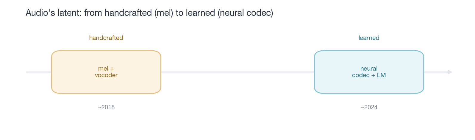
caption: “Audio’s middle latent finally went from handcrafted (mel + vocoder) to learned (neural codec). And that learned ‘codec’ is really a VQGAN-style learned VQ — the lingering name just obscures the shared origin.”

What this generation of audio codecs — SoundStream / EnCodec / DAC — did, viewed through the latent framing, is the audio counterpart of the JPEG → VQGAN history. Replacing the engineer’s handcrafted latent with a data-learned latent. This analogy is of course not perfectly precise (audio codec strongly inherits the engineering genes of compression-and-transmission, while VQGAN was designed from the start for downstream generation), but as a framing it’s clear.

A few details make the audio version of this transition read differently:

It was late. VQGAN was 2021, SoundStream the same year — but for an audio learned codec to truly become the default front-end of downstream generative models, it had to wait until EnCodec 2022 + VALL-E/MusicGen 2023. A two-year gap isn’t large, but the speed at which the community accepted that “the handcrafted latent should exit” was slightly slower in audio than in vision.

It kept the name “codec.” It wasn’t called “audio VQGAN.” This naming continuity partly obscured its shared origin with image VQGAN — people treated it as “the next generation of compression engineering,” not “the next generation of generative models.” This framing bias influenced an entire generation of codec design choices (§2.1 will expand on this).

Its engineering template is more convergent. SoundStream / EnCodec / DAC are highly similar in architecture — convolutional encoder + RVQ + multi-discriminator — narrower in diversity than the image codec generation. This is the price of audio’s stricter perceptual constraints.

But the story has one more reversal: mel didn’t actually exit. The learned latent took over the “compress-recover” layer, but if you flip through the recent batch of audio tokenizers and generative systems, you’ll find mel coming back again and again in another identity — not as the final representation, but as the object being tokenized, or the target being predicted/reconstructed. dMel directly quantizes mel’s frequency bands into tokens; a large batch of flow-matching / diffusion systems (Grad-TTS, Matcha-TTS, E2-TTS, MELLE, and even the just-mentioned TML-Interaction) simply generate on mel; many codecs’ training objectives also carry a mel-reconstruction loss.

Why does mel keep coming back in modern audio generation systems? Because the few properties it carries are largely what a “well-modelable intermediate representation” needs: clean structural information — on the time-frequency grid, phonemes, harmonics, and the energy envelope are clearly visible, and the semantic structure is accessible at a shallow level; friendly as input — a regular 2D structure, low dimensionality, a stable distribution, easy for neural networks to model; easy as a prediction target — adjacent frames are highly correlated and the context is continuous, so the model’s uncertainty in predicting the next frame is naturally small. These three together are largely the early form of the “modelability” toolbox of §2.5 — except mel assembled it by hand, decades in advance. So rather than saying the learned latent replaced mel, it’s better to say they have been continually rediscovering the benefits mel already had, and trying to push those benefits to the extreme through learning.

Connecting this thread to what follows makes it flow naturally: §2’s discrete direction = the mel + vocoder paradigm replaced by “learned discrete latent + audio LM”; §3’s continuous direction = the mel + vocoder paradigm replaced by “learned continuous latent + diffusion/flow matching.” The two directions are actually solving the same thing — replacing the handcrafted latent with a learned one. Their divergence is only in the second-stage modeling tool (LM vs diffusion/flow) and the first-stage latent type (discrete vs continuous). §4 will argue that these two divergences are actually converging toward the middle.

But standing in this section, first seeing clearly what the first widely used latent was, what was good about it, and the logic by which it was replaced — only then is the foundation for all subsequent discussion solid.

2. The Discrete Direction: Audio as Language

If the continuous direction is about adapting Sander’s “latents are high-level pixels” narrative onto audio intact, then the discrete direction’s ambition is a bit larger — it tries to turn audio largely into another kind of text. Tokens, vocabularies, autoregression, in-context learning — these concepts tailor-made for language models, once taken over by audio, are not a simple engineering analogy. The possibility they bring is: letting “understanding a sound” and “speaking a sound” share one underlying representation, thereby bypassing the vision-domain pattern of “understanding goes through CLIP, generation goes through latent diffusion,” where each walks its own road.

This is a very ambitious bet. This section advances along the engineering mainline of SoundStream → EnCodec → DAC; along the way it spends quite a bit of ink discussing why RVQ became the default choice for most audio codecs, and why the AudioLM paradigm had to invent the strange audio-specific division of labor “semantic token + acoustic token” — and why this “two tokenizers” engineering form is being absorbed into a single codec. It finally ends with a few typical downstream LM modeling patterns (VALL-E, MusicGen, Moshi) and ends with a Observation. But this Observation is more restrained than what I originally set out to write — whether the discrete direction’s bet pays off is still unclear today.

2.1 From VQ-VAE to SoundStream / EnCodec / DAC

This line of discrete audio codec research should have happened back in 2017, but was four years late.

The original VQ-VAE paper already had speech — van den Oord et al. 2017⁸ demonstrated on VCTK that the learned discrete codes could retain the spoken content and discard the speaker identity. This is practically the early form of the entire later “semantic vs acoustic” line of thinking. The basic idea was already there. But over the next four years, no one pushed it into something usable.

Why? Three things blocked the way, and each was very real. The waveform is too long — 16 kHz is sixteen thousand samples per second, and quantizing directly on the waveform makes it very hard to compress the bitrate down to a range an autoregressive model can handle; Jukebox (OpenAI, 2020)⁹ made an early large-scale attempt on music with a three-level multi-resolution VQ-VAE, proving that “audio really can be turned into tokens and then modeled with an LM,” but sampling was too slow to be usable and artifacts were clearly audible. mel + vocoder was already good enough — during 2018 to 2021, the TTS community’s attention was largely on the two-stage Tacotron / FastSpeech + HiFi-GAN paradigm, the handcrafted latent was working smoothly (§1.2 explained why), and there was no pressing reason to switch. The downstream engineering stack hadn’t grown up yet — in 2020, transformers were far less efficient at processing long sequences than today, and audio tokens are hundreds per second, which nobody wanted to feed to the models of that time.

The turning point was SoundStream (Zeghidour et al., Google, 2021)¹⁰. Its most important contribution wasn’t any single trick, but cleanly porting the engineering framework of the “codec” into neural audio — it wasn’t the earliest neural audio compression (Kleijn 2018 had already tried), but it was the first to make this line into a clear, reusable template: a convolutional encoder/decoder end-to-end, with reconstruction, adversarial (multi-scale STFT discriminator), and a bitrate constraint all combined in the objective function. Once the template was established, the entire subsequent generation of work grew according to it. Two recurring components were buried in the template: RVQ (residual quantization, important enough, saved for 2.2 to discuss separately) and quantizer dropout (one model supporting multiple bitrate tiers, the origin of scalable bitrate).

EnCodec (Défossez et al., Meta, 2022)¹¹ made this template much more practical — adding LSTM, extending to 24 kHz full-band and 48 kHz stereo, with open-source code and weights. Open-sourcing was decisive: the immediately following VALL-E and MusicGen took EnCodec directly as their front-end. As long as a codec is free and easy to use, it will become the default dependency of an entire generation of downstream work within a year or two — we’d already seen this pattern appear once in vision when VQGAN spread.

Then came DAC (Kumar et al., Descript, 2023)¹², one of the strongest general-purpose codecs in current reconstruction quality: snake activation introduces a periodic bias, multi-scale + multi-period discriminators, factorized + L2-normalized codebooks, pushing the objective reconstruction quality at low bitrates like 6 kbps up another notch.

But DAC highlights an important detail — because it’ll keep coming back. DAC’s optimization objective leans toward perceptual quality, not waveform fidelity. On music and general audio, the SI-SNR it reconstructs is even negative: viewed sample-by-sample, the difference between the reconstructed signal and the reference is larger than pure noise; yet perceptual metrics like ViSQOL and UTMOS are still high. This isn’t a bug, it’s a design philosophy — a codec trained with a perceptual GAN essentially does perceptually equivalent re-synthesis: it sounds identical to the ear, but the samples are re-synthesized, the phase is rewritten, the transients are micro-adjusted, and the time domain isn’t strictly aligned at all.

Why did DAC move in this direction while EnCodec didn’t? The root is in the loss balance. Among the set of codec-training losses, the only one that truly forces “waveform samples to align with the reference” is the time-domain L1 — mel L1 looks only at magnitude and discards phase, the multi-scale STFT discriminator only requires “looks real” not point-by-point alignment (the discriminator seeing phase ≠ forcing phase alignment), all phase-tolerant. EnCodec deliberately uses a Loss Balancer to hold down the time-L1 gradient so the adversarial terms don’t overwhelm it; DAC has no such gate and additionally adds a phase-invariant multi-period discriminator and the periodic bias of Snake activation — so the optimization naturally slides toward the solution of “satisfy all phase-tolerant terms, give up sample alignment,” which is re-synthesis.

The real significance isn’t DAC, but how to read codec benchmarks: sample-level metrics (SI-SNR, SDR) on a perceptual-loss codec measure the metric’s mismatch with the codec’s design philosophy, not the codec’s ability — DAC’s source-separation SI-SDR looks worse, but switch to perceptual MOS or ASR-on-separated-speech and the conclusion may flip. Remember this metric bias — it comes back in §3 and §4 when comparing continuous and discrete; many “discrete loses to continuous” conclusions carry it. Conversely, DAC’s preference makes its tokens preserve timbre, formants, and the energy envelope, so on timbre-dependent downstream tasks like speaker recognition it’s actually stronger than EnCodec (clearly visible on the DASB benchmark¹³).

Putting SoundStream, EnCodec, and DAC together, one thing is worth noting: they are very similar. The convolutional encoder downsamples the waveform 2× per level down to 50 or 75 Hz, attaches an RVQ bottleneck, then convolves symmetrically back up; the loss is often the same set of reconstruction + adversarial + commitment. This convergence isn’t largely a good thing — what it indicates isn’t that “the problem is solved,” but that the whole design is being dragged by a very narrow objective (multi-band reconstruction quality + fixed bitrate), and once that objective is accepted, the remaining room to maneuver is nearly gone.

Behind this is the design bias implied by the word “codec”. It comes from audio coding — the MP3, AAC, Opus lineage — whose core concern is the duality of compression and recovery. This is closely related to the opposite of image VQGAN’s origins: VQGAN was born from the start for “making the latent easy to model with an LM,” with reconstruction merely the means. Audio codecs were from the start more engineering-oriented, more fixated on perceptual quality, treating downstream modelability as a secondary consideration.

This obsession with perceptual quality has a deeper root: audio’s flaws are harder to forgive than images’. In an image, a patch of texture being slightly off, the color shifting a few shades — the eye sweeps past and lets it go; vision has a high tolerance for local static errors. But audio flows, and the ear is extremely sensitive to certain classes of distortion: a click, a frame of buzzing, a misplaced harmonic — it instantly jumps out of the continuous auditory stream, and once perceived, it is hard to ignore, the texture of the whole stretch collapsing. This is why the audio community holds MUSHRA / MOS subjective listening tests as the gold standard, and why codec designers would rather stack four or five discriminators to strongly enforce perceptual quality — in audio, “reconstruction off by a little” is often not a slight quality dip, but an artifact directly exposed.

This origin shaped its preferences and also circumscribed its blind spots — for instance, near-zero exploration of variable-length tokenizers, a point left for §4 to discuss in detail.

2.2 The popularity of RVQ: why most audio codecs choose residual quantization

RVQ is the most “audio-flavored” design choice of this generation of audio codecs. Its presence is so strong that if you open any discrete-audio paper from after 2022, the first figure almost always contains that hierarchical-residual box. Mousavi et al.’s survey¹⁴ lists around 55 discrete audio tokenizers, more than half of which use RVQ or its variants; the rest are basically challenging some specific pain point of RVQ, rather than building an largely different system.

Why is it needed?

Consider a 24 kHz audio, convolutionally downsampled 320× to a 75 Hz frame rate. One frame with a single-layer VQ, codebook size 1024, is 10 bits per frame, a bitrate of 750 bits/sec ≈ 0.75 kbps. This bitrate is far from enough for speech perceptual quality — the lower bound for intelligible human speech is around 2–3 kbps, and high-fidelity recovery generally needs above 6 kbps.

The intuitive solution is to enlarge the codebook: raise 1024 to 16384 or even 65536. But a single-layer VQ, when the codebook is large (especially beyond a few thousand), is more prone to codebook collapse / declining utilization — a large number of codewords are never selected, and the effective capacity is far below the nominal capacity. The exact threshold depends on the training data scale, encoder capacity, commitment loss, and codebook-update strategy. RVQ’s solution is to split capacity into layers. The first-layer codebook quantizes the original latent, the second-layer quantizes the first layer’s residual, and so on. After N layers, the final reconstruction is q₁ + q₂ + … + q_N. Each layer’s codebook faces only the distribution of its own layer’s residual — smaller and smaller in magnitude, finer and finer in structure — so no codebook needs to be too large; size 1024 is enough. 8 layers × 10 bits = 80 bits/frame × 75 Hz = 6 kbps, exactly reaching the high-fidelity range.

RVQ’s byproduct: hierarchical semantics

The truly interesting thing about RVQ isn’t capacity itself, but the unexpected side effect the hierarchy brings: the first-layer codebook naturally takes on coarse information — fundamental frequency, phoneme outline, overall energy; subsequent layers gradually encode timbre details, phase, transients, noise. This hierarchy isn’t a design goal; it’s something that naturally emerges under optimization pressure — the first layer, to maximize reconstruction within the fewest bits, must grab the most discriminative signal.

This side effect determines the pattern of subsequent downstream modeling. The reason AudioLM¹⁵ introduced a separate semantic-token stream, and the reason Mimi can push semantic information into the first RVQ layer through WavLM¹⁶ distillation, is that audio benefits from an explicit hierarchy between content and acoustic detail. 2.3 will expand on this.

The cost

The sequence length goes from T to T × N. A 30-second, 75 Hz, 8-layer RVQ audio is 30 × 75 × 8 = 18000 tokens. This forces the downstream LM to adopt a “non-trivial” unrolling scheme — VALL-E separates the first layer from the rest (AR + NAR), MusicGen uses a delay pattern to let multiple layers be predicted in parallel, UniAudio/Moshi use a local transformer to do a small AR over the codebook dimension. 2.4 discusses these patterns specifically.

A small landscape of quantization methods

Although RVQ dominates, the actual landscape of quantization algorithms is much richer than the “RVQ vs lookup-free” dichotomy. A few representative ones (the fuller eight-category split is in the survey):

• SVQ (Single VQ) — a single large codebook (WavTokenizer¹⁷, BigCodec¹⁸, TS3-Codec¹⁹, dMel²⁰). The bet: one token per frame keeps the downstream LM’s unrolling trivial — no delay pattern, no local transformer. The cost: a single codebook carries only limited information per frame (log₂4096 ≈ 12 bits), so it needs a bigger encoder/decoder and a higher frame rate to hold quality (WavTokenizer 75 Hz, BigCodec 80 Hz). Push it to 40 Hz and reconstruction degrades noticeably — “low frame rate + single codebook” has a floor, and reaching Mimi’s 12.5 Hz seems to require multiple codebooks.
• RVQ — hierarchical residual, the aforementioned mainstream.
• MSRVQ (Multi-Scale RVQ) — SNAC’s²¹ approach: RVQ layers run at different temporal resolutions (coarse structure at a low rate, detail at a high rate — 12 / 23 / 47 Hz), a way to get variable-rate inside the RVQ framework. Our LLM-Codec²² adds a twist: its codebook is taken directly from an LLM’s word embeddings (§2.3), so the multi-scale tokens are also “aligned to the text vocabulary” — layered by granularity and looking like text to the LM at once.
• FSQ (Finite Scalar Quantization)²³ — quantizes each dimension independently to fixed discrete levels, with no nearest-neighbor lookup and no collapse. In vision, MAGVIT-2 and others use it very successfully. In audio, SQ-Codec, Spectral Codecs, HARP-Net, etc. use it — and notably, the survey’s controlled ablation found FSQ on 16 kHz actually surpasses RVQ on UTMOS/DNSMOS, so at the perceptual level FSQ doesn’t necessarily lose.
• A few others just refine one specific part of RVQ rather than building a different system: GRVQ (HiFi-Codec²⁴ splits the latent into groups, each doing RVQ, to ease first-layer overload), CSRVQ (ESC²⁵ refines progressively across encoder/decoder levels), PQ (sub-vector quantization, common in SSL models like Best-RQ²⁶), and the “k-means on a pretrained SSL model’s hidden features (HuBERT²⁷, etc.)” route — SSL-as-encoder + post-hoc discretization, not really a codec (see §2.3).

Let me return to fill in the foreshadowing left by SVQ above. We said “a single codebook must go high frame rate to keep quality,” but this floor has a premise: it holds under the setting of “directly reconstructing the waveform.” Once you switch the target to mel — directly tokenizing mel, or having the decoder reconstruct mel — the difficulty immediately drops a notch: mel is low-entropy, phase-free, and contextually continuous (those nice properties of §1.2), and quite a few works can compress a single-layer VQ down to 25 Hz, leaving waveform reconstruction to a separate vocoder. This is another piece of evidence that mel didn’t really exit — it shifts the line of “how low a single codebook can compress” down a notch.

Why is audio still mostly RVQ? This question must first distinguish which layer is being asked about.

If the question is about the codec itself — the end-to-end “waveform compressed into tokens, then recovered back into waveform from tokens” — then RVQ is indeed still mainstream, for three reasons.

First, and most concrete: RVQ can get high fidelity and low frame rate at the same time. These two things are contradictory for a single-layer VQ — as said earlier, a single codebook must push the frame rate up to keep quality (WavTokenizer 75 Hz, BigCodec 80 Hz). RVQ stacks capacity with hierarchical residuals, so it can recover high-fidelity audio at a very low frame rate (Mimi 12.5 Hz). And the frame rate directly determines the downstream LM’s sequence length, so low frame rate = short sequence = good modeling, which is the most valuable gift a codec gives downstream. A single layer struggles to have it both ways.

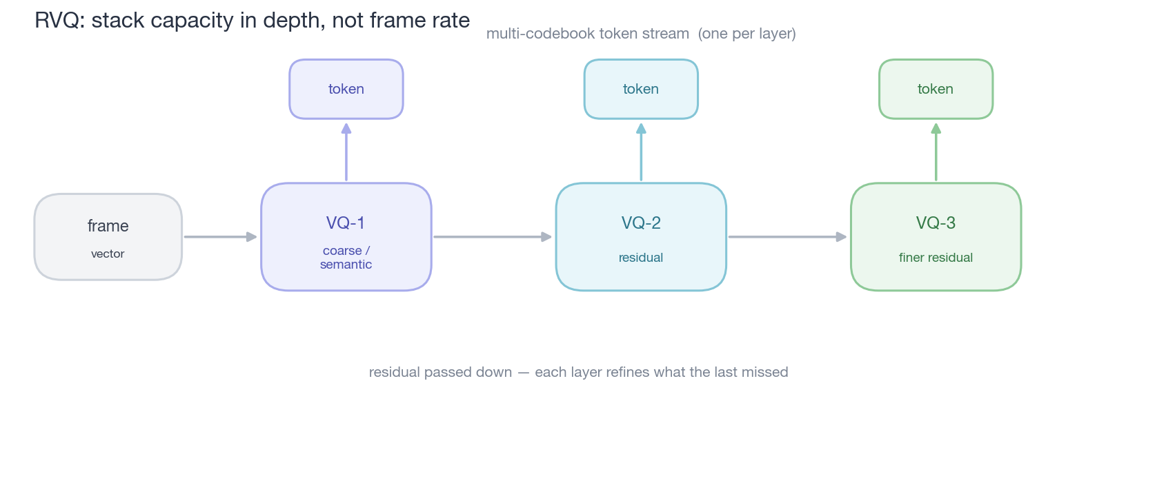
caption: “RVQ’s bet — build capacity in depth, not by raising the frame rate. The first quantizer is coarsest (carries semantics and most energy); each later layer quantizes the previous layer’s residual, adding finer detail; every layer emits one token, together a multi-codebook stream. So one frame can hold the information needed for high fidelity while the frame rate stays low — exactly where its value lies.”

Second, ecosystem inertia. EnCodec/DAC are free, easy-to-use pretrained codecs, and around multi-layer RVQ a whole set of downstream recipes was accumulated (delay pattern, local transformer, training tricks), which new work just picks up and uses. Incidentally, let me clear up a common misunderstanding: switching to single-layer SVQ doesn’t require “redesigning” downstream — quite the opposite, it directly simplifies it away (one token per frame, fed directly to a standard causal LM, delay pattern removed). So SVQ’s cost isn’t on downstream, but on the codec side, in that “fidelity × low frame rate” dilemma — which loops right back to the first reason.

Third, the more essential reason: RVQ’s hierarchy is structurally free, and no other scheme has it. FSQ/LFQ’s dimensions are semantically equivalent, and SVQ is a single codebook with no hierarchy at all — to do semantic / acoustic decoupling, you can only force it with extra training objectives. Once you lose this free hierarchy, the entire design philosophy of the AudioLM family — “first layer for semantics, later layers for acoustics” — has to be redone. Vision can afford this redo (there, semantic / acoustic decoupling isn’t a core need), but audio can’t — this point is the core argument of the judgment in §4.2.

But if the question is “are today’s mainstream audio generation systems still using RVQ,” the answer is much more subtle. The batch of production-grade TTS systems from the past year — CosyVoice, Seed-TTS²⁸, etc. — are increasingly actively bypassing the multiple-codebook thing: the first stage uses a single-layer semantic VQ (or supervised phonetic token) for autoregressive content generation, and the second stage uses flow matching or diffusion on mel / continuous latents to generate acoustic detail. In other words, AudioLM’s two-stage semantic + acoustic paradigm hasn’t disappeared, but the acoustic stage has been swapped from SoundStream RVQ to “continuous representation + non-AR decoder.” RVQ’s “hierarchical semantics” has been substantively dismantled: the first layer’s content duty is taken over by a single-layer supervised VQ, and the later layers’ acoustic-detail duty is taken over by a continuous decoder — the whole multiple-codebook unrolling machinery (delay pattern, local transformer) removed largely.

The appeal of this design isn’t just “bypassing RVQ.” The deeper motivation is to minimize changes to the LM architecture: one token per step, standard causal autoregression — exactly the same as a text LM. This means you can directly reuse all the off-the-shelf dividends like the LM’s KV cache optimizations, without having to redesign the transformer structure specifically for audio. The acoustic complexity is outsourced to a separate flow matching head, keeping the main LM clean. This is the discrete direction’s most thorough embrace of the “tokens are flexible” argument — since the token stream can be anything, make it as much like the text token stream as possible, and hide audio’s specialness in modules outside the LM.

So the more accurate judgment is: RVQ remains mainstream at the codec-design layer, but at the end-to-end generation-system layer it’s being squeezed by the “single-layer semantic VQ + continuous decoder” direction. This hybrid direction will reappear in §4.2 — it’s the strongest evidence that the “continuous features take over the generation side” direction has already run successfully in products.

Takeaway: RVQ isn’t just a compression trick — it also hands the downstream LM a useful hierarchy: early layers lean semantic, later layers acoustic, and the same token stream can be consumed on demand. That, more than compression, is why it’s hard to replace in generation systems.

2.3 AudioLM’s semantic / acoustic paradigm

In one sentence: AudioLM splitting tokens into semantic + acoustic was a 2022 expedient — the insight (long-range semantics need to be carried separately) is right, but the implementation, “two independent tokenizers + a three-stage cascade,” is now being folded into a single codec. Below I trace how it came about and how it got absorbed into one codec.

Back to Google Research in 2022. A group of people was doing a concrete experiment: take SoundStream’s RVQ tokens, train a standard autoregressive transformer, and see if they could continue a speech prompt into longer speech.

The experiment ran very well — until a few seconds in.

The model’s reconstruction quality was mostly fine; every frame sounded like a real person speaking. But the topic started to drift. The speaker would suddenly jump to irrelevant content, occasionally degenerating into a meaningless stream of syllables — a very strange phenomenon: acoustically mostly reasonable (every sound is human-like), semantically mostly derailed (what’s being said starts to mean nothing).

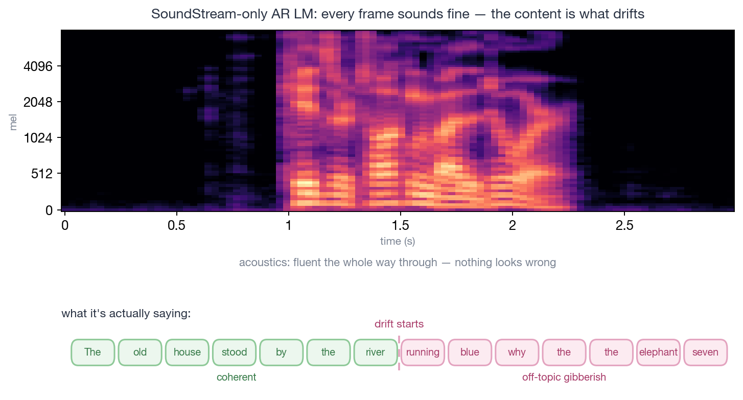
caption: “The drift you get from a pre-AudioLM SoundStream-only AR LM. The spectrogram on top shows the acoustics stay fluent the whole way through — every frame sounds like real speech, nothing looks wrong; the problem is largely in the content below — coherent at first (green), then derailing into off-topic gibberish from some word onward (red). Acoustically fine, semantically off the rails — that’s what drift is.”

This isn’t hard to diagnose. SoundStream is a codec — it optimizes “how to recover the waveform,” not “what the signal is saying.” Its tokens encode information that’s highly physically correlated between adjacent frames (the waveforms of adjacent 50 Hz frames are nearly identical), but the model is not explicitly told it what “finishing a sentence” means. At short distances the LM can learn the local connections between tokens (this frame to the next), but at long distances there’s no anchor telling it “we’re still talking about the same thing.”

If you only have this one kind of token, this is as good as it gets.

The AudioLM team’s solution was a bit roundabout. Rather than fixing SoundStream, they bypassed it and added another kind of token: cluster the intermediate-layer features of w2v-BERT (a self-supervised speech encoder)²⁹ with k-means to get a second discrete token stream — they called it the semantic token. This token performs well on the linear probing of phonemes and words — that is, what it encodes is “what the sound is saying.”

Then their model became a three-stage cascade:

First stage, the semantic LM — looks only at the semantic tokens, autoregressively generating content. This line is short and long-range stable, equivalent to “deciding what to say first.” Second stage, the coarse acoustic LM — given the semantic tokens as condition, predicts the first few layers of SoundStream RVQ (determining timbre, prosody). Third stage, the fine acoustic LM — given the coarse as condition, predicts the remaining layers (detail). Finally, the SoundStream decoder recovers the waveform.

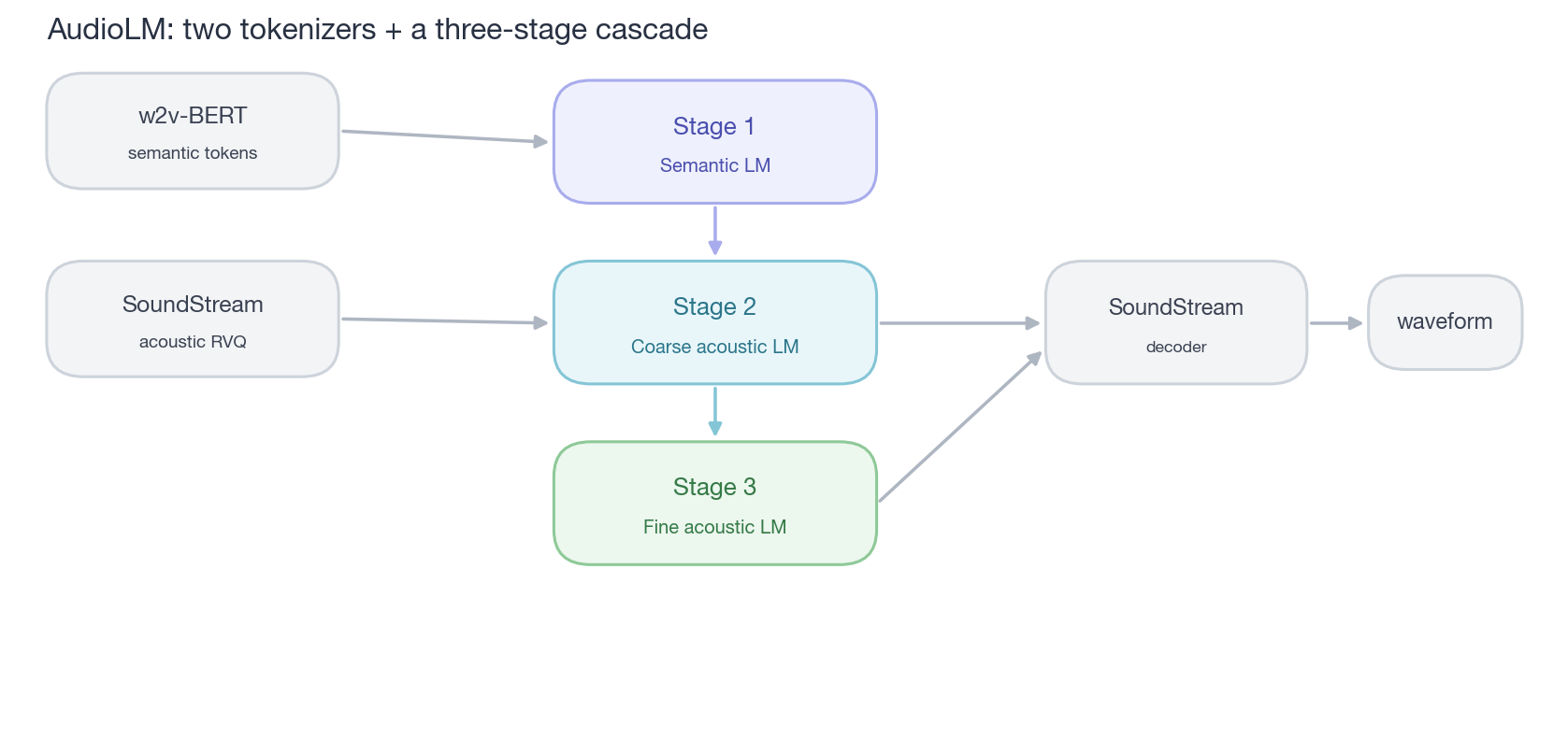
caption: “AudioLM’s cascade — two tokenizers + three LMs (the orange→blue→green three stages). Complex but effective: long-range semantics are anchored by the semantic LM, acoustic detail is filled in by the acoustic LM.”

This was effective. AudioLM could generate 30 seconds or more of coherent English babble — the longest free speech generation of 2022. Follow-up work like Bark, MusicLM, and VALL-E all borrowed inspiration from this paradigm. It became the standard recipe of those couple of years.

But this recipe is a bit strange.

There’s no equivalent in vision. No one would use a “semantic VQGAN” plus a “texture VQGAN” and then do a three-stage cascade — VQGAN’s tokens are enough. Why does audio have to be this troublesome? I can think of three layers.

The most fundamental layer: an image’s semantics is a static single point, while speech’s semantics is a trajectory unfolding over time. Generating an image, there’s only one semantics from start to finish — “a cat sitting on a sofa,” with all tokens serving the same static scene; there’s no such thing as “semantics evolving as generation proceeds.” Speech is different: what’s said every second is moving forward, the first stage of a sentence determines the second stage, this sentence determines the next — generating audio simultaneously requires continuous semantic planning. A vision LM doesn’t need the ability of long-range semantic stability, because there’s no semantics flowing over its “long range” at all; an audio LM must have it, otherwise it’s the drift we saw.

The second is sequence length. A 30-second audio, once unrolled, is a thousand-plus tokens, a long-context challenge for an LM; vision’s 16×16 latent is far shorter than this, and attention stabilizes easily. Audio needs a long-range anchor.

The third is the physical coupling of content and acoustics. Certain token changes that are acoustically small locally (subtle vowel-quality differences, consonant voicing differences, etc.) can correspond to largely different word meanings; conversely, a great many obvious acoustic differences (speaker, speaking rate, emotion, reverberation) don’t change the textual semantics at all. Tokens and “information” aren’t in bijection. Training an acoustic-only LM on such a deeply coupled signal, it can’t grow “semantic stability” by itself — because the signal simply doesn’t separate out the “semantic” dimension.

So AudioLM adding semantic tokens is essentially attaching, to a token stream that originally had no semantic dimension, a dedicated channel for carrying the “semantic trajectory” — using an engineering approach to supply the very ability that doesn’t exist in image generation but is essential in audio generation.

These three layers are actually the same information-theoretic principle. Split audio by conditional entropy: one half is low-entropy — content / semantics, nearly nailed down by context; the other half is high-entropy — timbre, phase, texture, the acoustic detail that’s “still random given the content” (which is exactly the part the semantic features are trained to throw away). And the irreducible loss of an autoregressive model at each step is exactly the conditional entropy \(H(z_t \mid z_{<t})\): the low-entropy half the LM predicts stably and accurately (the same reason text LMs are easy to train — text is a representation with extremely low conditional entropy), while the high-entropy half, forced onto the AR to “predict” frame by frame, either can’t be learned or drifts — the mathematical root of that SoundStream-only crash. So AudioLM adding semantic tokens essentially makes this entropy decomposition explicit: hand the low-entropy, predictable half to the LM to predict, and hand the high-entropy, random half to the acoustic model to generate — predict the predictable, generate the rest. It’s worth emphasizing the second stage: the high-entropy detail isn’t “predicted” accurately, it’s “sampled” out by a random generator — forcing the AR to losslessly predict it is using the wrong tool to begin with.

This principle outlives AudioLM itself: whether folding the division of labor into a single codec (RVQ first layer carries semantics, residual layers carry acoustics) or the continuous direction’s “semantic latent + generative decoder,” what they all do is the same entropy decomposition, just with a different implementation. So what’s to be dismantled below has never been this principle, but its complex 2022 implementation.

If you track the audio codec / audio LM work of 2024-2025, you’ll find a clear trend: new work almost all attempts to replace AudioLM’s two-tokenizer splice with a single codec. Mousavi et al.’s survey (2025-09) even says directly in its introduction that the acoustic vs semantic dichotomy is “insufficient” — because a great many acoustic codecs have been shown to carry semantic information (Mimi, SpeechTokenizer, dMel), while semantic tokenizers are also widely used for generation tasks (GSLM, TWIST, etc.). The two categories actually overlap. So they directly discard the dichotomy and switch to a finer five-dimensional taxonomy.

This doesn’t mean AudioLM’s insight was wrong — the intuition that “long-range semantics need to be specially carried” is correct. The problem is that “carrying” doesn’t necessarily require two independent tokenizers and a three-stage cascade. It can be done inside one codec.

There are four concrete paths to do this, understandable as “how to fold AudioLM’s two tokenizers into one”:

The first is distillation — making a certain layer of the codec explicitly carry semantics. SpeechTokenizer (Zhang et al., 2023)³⁰ was the first to do this systematically: when training RVQ, add an auxiliary loss to align the first-layer codebook’s output with HuBERT features. The result is that the first layer is “forced” to carry phonetic content, leaving later layers free to learn acoustic detail. Mimi (paired with Moshi, Kyutai 2024)³¹ pushed this path to the extreme — a 12.5 Hz frame rate, WavLM distillation into the first layer, causal convolution streaming-friendly, 8-layer RVQ × 2048 codebook ≈ 1.1 kbps (clearly lower than EnCodec’s 6 kbps range).

The second is hybrid encoder — using two encoders but fusing into one codec. X-Codec / SemantiCodec³²³³ are representatives: a dual-encoder, one branch ingesting SSL features, the other acoustic, fused and then quantized into a single token stream. This path is simpler in engineering than AudioLM (still only one kind of token for the downstream LM), but at the encoder level it acknowledges that “semantic and acoustic information have different sources.”

The third is supervised semantic — not distillation, but directly supervising with ASR. This path deserves a few more words, because it has an essential difference from the first two.

The representative work is CosyVoice’s S3 tokenizer³⁴ (Du et al., 2024): take an ASR model, insert a VQ bottleneck in the middle of the encoder, and train the whole model end-to-end with the ASR loss (CosyVoice 2 swaps VQ for FSQ for better codebook utilization). The token is semantic because it must support the latter half of the network in completing text recognition — the supervision signal comes directly from the transcript, no SSL teacher needed.

Note the essential difference between this design and the first two paths: S3 has no reconstruction objective; it isn’t a codec at all. SpeechTokenizer / Mimi are still codecs — they have a decoder, a reconstruction loss, and the semantic supervision is layered on top, the token having to both carry semantics and support reconstruction. S3 is a quantized ASR intermediate layer — it has no reconstruction objective, and what’s stripped by design is mainly speaker timbre (content and a good deal of prosody / rhythm actually remain in the token); “recovering the waveform from the token” is entirely outsourced to the downstream flow matching decoder. This also explains why CosyVoice necessarily grows into a “token LM + flow matching” two-stage form: there’s no timbre in the token at all, so it must be supplied back from the reference audio / speaker embedding at the flow stage.

Closer to codec form within the same direction is PAST (Har-Tuv et al., 2025)³⁵ — it retains the full codec structure (RVQ + reconstruction loss) and layers phonetic classification and ASR-CTC auxiliary losses on the first RVQ layer. Understand it this way: PAST is “codec + supervised semantics,” S3 is “ASR + quantization bottleneck” — the former retains waveform-reconstruction capability, the latter simply doesn’t reconstruct and outsources that job entirely. The two trade-offs correspond to different downstream forms: PAST’s tokens can still directly reconstruct the waveform, while S3’s tokens must be paired with a generative decoder.

The fourth is the most radical — disentanglement, splitting the latent into multiple parallel codebook streams. FACodec (NaturalSpeech 3’s codec, Ju et al., 2024)³⁶ trains four independent RVQ modules: content / prosody / timbre / acoustic detail, each supervised by a different loss. TiCodec, LSCodec³⁷, SoCodec, SD-Codec³⁸, etc. are different variants of the same idea — splitting by time-invariant (timbre) vs time-varying (content), by speaker vs content, by sound-source type. This path gives up the simplicity of “implicitly emerging hierarchy” in exchange for the controllability of “every codebook being interpretable.”

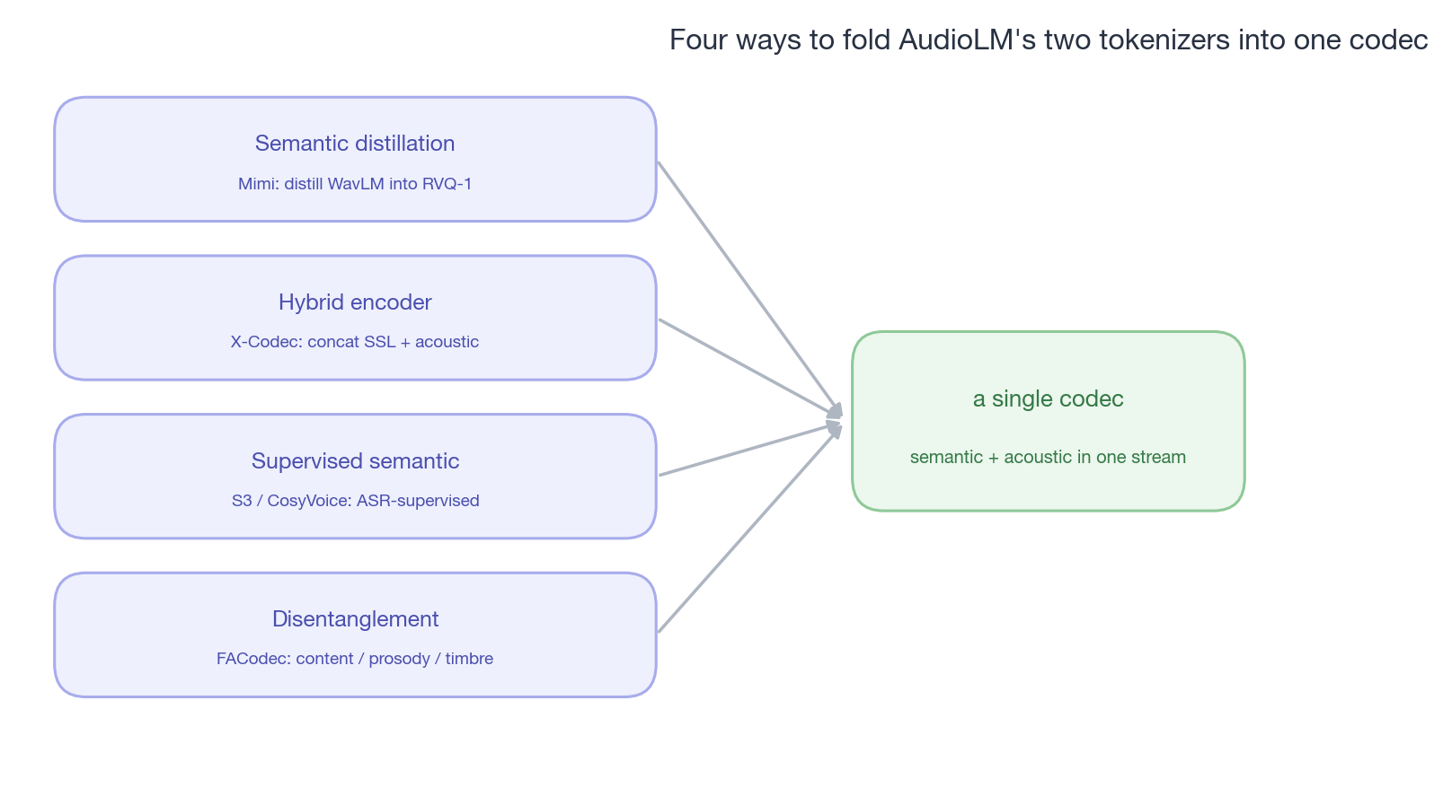
caption: “Four ‘replacements’ for AudioLM’s cascade. Different paths but a shared goal — fold the two tokenizers into one, so the downstream LM no longer needs a cascade.”

Worth mentioning: these four paths aren’t mutually exclusive. FACodec internally uses distillation and supervised loss too; Mimi internally has streaming design too. They’re more like four different “access points,” letting SSL/semantic signals seep into different positions of the codec.

2.4 Common patterns for downstream modeling

Given a multi-codebook RVQ token stream, how does downstream ingest it? This is where audio-generation engineering has changed most frequently over the past three years. There are two axes here: one is how to unroll the multiple codebook layers (designs within the AR framework — the four examples below embody the evolution from “two models” to “a single model”); the other is whether or not to be autoregressive at all (AR vs non-autoregressive, discussed separately in the latter half of this section). Look at the first axis first.

VALL-E (Microsoft, 2023)³⁹. Core problem: EnCodec has 8 codebook layers per frame — how to autoregress? The answer is concise — only the first layer uses AR, the remaining 7 layers use NAR. The AR transformer autoregresses on the first-layer codebook (this layer carries content and prosody, and AR guarantees long-range structure), and the NAR transformer predicts the remaining 7 layers in parallel. Inference is fast (the AR-part sequence is 8× shorter than flat) and conveniently unlocks zero-shot voice cloning. The cost is two independent transformers, hard to share.

MusicGen (Meta, 2023)⁴⁰ — delay pattern. The N codebook layers aren’t predicted in parallel at the same moment, but are staggered by a delay: at t=0 output c0, at t=1 output c0+c1, at t=2 output c0+c1+c2… each step simultaneously outputs all current layers, but each layer’s “time” is offset by i steps. This is equivalent to “AR over time + partial AR over codebook.” A single transformer, sequence length = T, with no ×N cost. The first N-1 steps have slightly worse quality but it matters little in practice. After MusicGen, the delay pattern became a very influential class of design in multi-codebook autoregression — MusicLM, parts of Stable Audio’s implementation, and MAGNeT⁴¹ all bear traces of this idea; together with depth transformer / AR+NAR / parallel prediction and other directions, it forms today’s design space.

UniAudio (Yang et al.)⁴². This is the first work to unify multi-task audio generation under a single framework — over a dozen tasks like TTS, voice conversion, singing voice synthesis, sound generation, music generation, and speech enhancement share the same transformer, the same token vocabulary, and the same training objective. Its most important contribution to downstream modeling is the multi-scale transformer: on a multi-codebook RVQ input, use a global transformer to autoregress along the time dimension, plus a local transformer to autoregress over the codebook dimension within each frame. The global looks at long-range structure, the local at the within-frame hierarchical division of labor, and the two are connected through a frame-level summary token.

This architectural pattern has precedents like MegaByte in byte/character sequence modeling, but on audio multi-codebook, UniAudio is the first work to make it run — multi-task, scaled to ~1B parameters, with about 100k hours of training data. It showed that a single end-to-end LM can simultaneously play multiple audio-generation roles is feasible, without training a separate model for each task. This finds an echo in later systems like Moshi.

Moshi (Kyutai, 2024). Goes further, the system to date closest to “language-model-paradigm audio.” A few key designs:

• Mimi codec: a single codec, 12.5 Hz frame rate (6× lower than EnCodec’s 75 Hz), first-layer WavLM distillation. This 12.5 Hz isn’t an optimization detail, it’s a game changer — it cuts the total token count of a 30-second audio from eighteen thousand to three thousand, making “modeling audio end-to-end with an ordinary LM” truly feasible in terms of compute.
• Inner monologue: text tokens and audio tokens are interleaved along the time dimension — the model simultaneously generates “the text of what it’s saying” and “the audio it actually speaks,” with text as high-level planning and audio as the actual output. This design responds to AudioLM’s semantic/acoustic division of labor, but expresses it with a single token stream.
• Depth transformer: there’s a small AR over the codebook dimension — the main transformer unrolls over time steps, and within each time step a small transformer sequentially predicts the 8 codebook layers. Moshi’s contribution is assembling it together with streaming, inner monologue, and a low-frame-rate codec into a complete real-time dialogue system.
• Full-duplex: the user’s and the model’s audio streams are two independent channels, with the model listening and speaking simultaneously. This is the real-time interaction requirements shaping the representation — only a streaming codec + streaming LM can do it.

CosyVoice / Seed-TTS: discrete + continuous hybrid. An interesting bifurcation appears in the latest generation of TTS systems: the first stage discrete, the second stage continuous. The first half uses semantic-rich tokens (SSL-quantized or the first layer of a distilled codec) for autoregression (inheriting the LM paradigm: controllable, in-context learning, zero-shot); the second stage takes the discrete tokens as condition and uses flow matching or diffusion on continuous latents / mel to generate acoustic detail (inheriting the continuous direction: high quality, stable sampling). This is a phenomenon worth expanding on specifically — it shows the field has accepted a division of labor inside the generation pipeline: discrete tokens carry the AR / content-planning stage (benefiting from LM infrastructure — controllable, in-context learning, zero-shot), continuous flow / diffusion carries the acoustic detail (benefiting from high-quality and stable sampling). This is closely related to the engineering incarnation of §2.3’s “predict the predictable, generate the rest” entropy decomposition, and §4 will use it as the key argument that wraps up the whole article.

The second axis: discrete tokens don’t have to be generated autoregressively. The four preceding designs all circle within the AR framework, but discrete tokens can also be generated non-autoregressively — predict all positions in parallel at once, then iteratively refine a few steps. DiffSound⁴³ (Yang et al., 2022) is the earliest discrete diffusion on audio: discrete diffusion on VQ-VAE’s mel tokens, predicting all tokens in one step then progressively correcting, several times faster than an AR decoder. SoundStorm⁴⁴ (Google, 2023) ported MaskGIT’s confidence-based parallel decoding onto codec tokens, matching the quality of AudioLM’s AR generation while being two orders of magnitude faster (a 30-second audio out in 0.5 seconds). MAGNeT and NaturalSpeech 3’s³⁶ factorized diffusion also belong to this class. The trade-off of this axis is clear: trade parallel/iterative for speed — a few refine steps and the result is out, unlike AR which must walk T steps; the cost is non-causal (the whole sequence must be visible during generation), so it can’t do streaming and can’t eat the next-token dividends of text LMs. It’s actually spiritually akin to the continuous direction’s diffusion — discrete tokens borrow diffusion’s “iterative refine” generation mechanism, another example of the blurry boundary between discrete and continuous.

The direction of evolution is clear. Putting VALL-E (two models), MusicGen (delay pattern + single transformer), and Moshi (single codec + single transformer + streaming) on a timeline, the trend is very obvious: increasingly simplified, increasingly unified, increasingly like an “ordinary LM.” This also responds to Sander’s “tokens are flexible” — once the representation becomes tokens, all the LM’s engineering dividends (KV cache, speculative decoding, long-context optimizations, in-context learning) become directly usable. This is the discrete direction’s biggest irreplaceable advantage in product deployment.

2.5 The “modelability” toolbox of the discrete direction

This section is worth separating, because it’s the discrete direction’s most important hidden thread — more worth remembering than any single codec. Reading §2.2–2.4 all the way through, you’ll find: what codecs have truly accumulated over these years isn’t higher reconstruction quality, but a whole set of craft for “making the representation easier for downstream generative models to learn.” Sander’s original article calls this class of operations regularising for modelability. This is largely the most essential watershed between codecs after 2023 and the first generation of pure-compression codecs (the SoundStream/EnCodec batch): for the former, every design choice aims not at “how accurately to reconstruct” but at “how well the second stage learns.”

The toolbox on the audio discrete side is even larger than vision’s:

• Frame rate — the most important knob. Mimi makes 12.5 Hz a core selling point, TADA compresses to 2-3 Hz: the sequence length directly determines whether the LM can learn. Halving the frame rate halves the downstream LM’s context burden.
• Capacity configuration — more codebooks isn’t better: more codebooks improve reconstruction but add redundant dimensions and downstream-modeling burden, and often hurt downstream tasks like ASR / SE / SS. Capacity must be co-designed with the downstream consumption mode, not tuned by reconstruction metrics.
• Semantic supervision — distillation / supervised loss / disentanglement (§2.3’s four paths): make the token’s structure friendly to the LM, translating the “decoder’s private language” into a “public language.”
• Making tokens carry an autoregressive prior of their own — the AR prediction loss we proposed in ALMTokenizer⁴⁵: hang a lightweight continuous AR transformer on the RVQ latent, using the features of the first few codebook layers to predict the next layer (MSE optimized), writing “whether the downstream LM can predict accurately” directly into the codec’s training objective. The motivation is a very concrete observation — RVQ’s first layer leans semantic and is the easiest to learn, while the residual layers lean acoustic and are clearly harder for the AR to fit, and this loss specifically lowers the prediction difficulty of the residual layers. The cost is honest too: it slightly lowers reconstruction, in exchange for significantly improved prediction accuracy of the second and third layer tokens and a drop in downstream TTS WER. This is the cleanest example of this section’s theme: sacrifice a little reconstruction in exchange for downstream being easier to learn.
• The unrolling scheme — delay pattern, local transformer, AR+NAR division of labor: the same token stream, arranged differently, has wildly different modelability. Representation design doesn’t stop at the encoder; how tokens are “fed” is part of representation design too.
• Generative decoder absorbing quantization error — make the decoder a generative model rather than a deterministic recovery: LaDiffCodec’s diffusion decoder⁴⁶, CosyVoice’s flow stage are both this idea. Discrete tokens necessarily have quantization loss, and a deterministic decoder reconstructs the loss intact as an artifact, while a generative decoder takes the token as condition and samples out a reasonable audio realization — which amounts to relaxing the precision requirement on the upstream token, so the downstream LM doesn’t have to predict it down to the last bit. This is largely the interface where the continuous direction’s “generative reconstruction” is borrowed into the discrete direction.

Lining up these six tools, you’ll see they point at the same action: what they tune is all about “how well downstream learns,” not a single one aimed at reconstruction quality. This is the full engineering unfolding of the awareness of “designing representations for downstream” — and §3.3 will show the continuous direction holding a nearly mirror-image set of tools, answering the same question.

3. The Continuous Direction: Audio as Latents

The discrete direction’s story is “turning audio into another kind of text.” The continuous direction’s starting point is much plainer — porting the engineering template of image generation onto audio. But during the porting, two things no one anticipated happened: the latent started to carry semantics, and autoregression became possible without discrete tokens. This chapter discusses these two turns, and how they turned the continuous direction from a “conservative alternative” into another candidate for a unified audio interface.

3.1 First phase: adapting the vision template

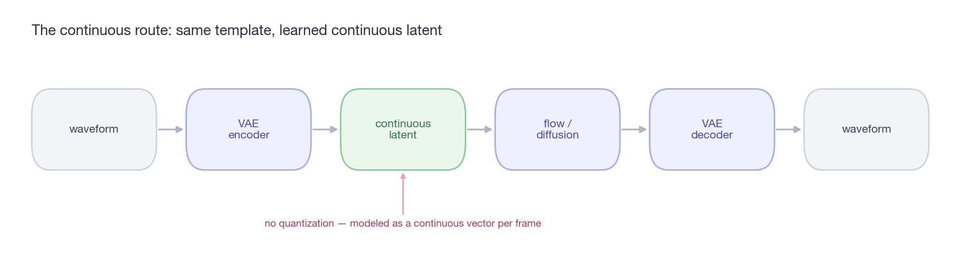
caption: “The continuous route’s engineering template is almost a port of the LDM diagram in §1: waveform → VAE encoder compresses to a continuous latent → flow / diffusion generates on that latent → decoder recovers the waveform. The only difference from the discrete route: the middle latent isn’t quantized — each frame is a continuous vector, not a codeword.”

First, let’s correct a common misunderstanding: sequence-latent models for audio appeared very early. VRNN (Chung et al., NeurIPS 2015)⁴⁷ was already doing speech modeling with one latent per time step on TIMIT / Blizzard, SRNN (Fraccaro et al., 2016)⁴⁸ followed up, and FHVAE (Hsu, Zhang, Glass, NeurIPS 2017)⁴⁹ used a hierarchical sequence VAE to achieve speaker/content disentanglement. The insight of “preserving the time grid” arrived six years earlier in audio than in vision’s VQGAN — because audio’s temporal nature is so obvious that no one would think to compress an entire utterance into a single fixed vector.

What slowed down the continuous direction wasn’t the grid, but the blur. The Gaussian likelihood of a pure VAE has a well-known problem: over-smoothing — repeatedly studied in the parametric-TTS era (Toda & Tokuda 2007’s⁵⁰ Global Variance compensation was largely fixing it), where the generated spectral trajectory is the average of all reasonable realizations, sounding muffled and dull. In the language of §1.1: the Gaussian likelihood forcibly regresses to the mean on texture, and the mean of a texture isn’t any legal texture.

The remedy converges with vision by a different road: put adversarial training into the decoder. The landmark of this step is VITS (Kim et al., ICML 2021)⁵¹ — its full name is often forgotten: Conditional Variational Autoencoder with Adversarial Learning for End-to-End TTS. Frame-level sequence latent + flow prior + adversarial decoder, it became one of the most widely deployed TTS architectures of 2021-2023. So “the VAE didn’t succeed in audio” is a false proposition — the VAE needed an adversarial decoder to produce sharper perceptual detail, the same lesson as vision training KL-VAE by the VQGAN recipe.

Then came the maturity of the porting. Diffusion models were first tried on the waveform (WaveGrad, DiffWave, 2020 — too slow), then ported onto mel (Grad-TTS, DiffSinger, 2021), and finally moved to a learned continuous latent: Make-An-Audio (Huang et al., ICML 2023)⁵² did text-to-audio general audio generation, and Stable Audio (2023-24)⁵³ ported the SDXL template onto music⁵⁴ — convolutional VAE + DiT, a continuous latent of around 64 dimensions at 21.5 Hz; Music2Latent (2024)⁵⁵ used consistency ideas to achieve single-step decoding. The generation side was taken over by flow matching: Voicebox (2023)⁵⁶ made this direction visible, with Matcha-TTS⁵⁷, SimpleSpeech 1/2 (Yang et al., 2024)⁵⁸, E2-TTS, and F5-TTS (2024)⁵⁹ following — a more direct training objective and fewer sampling steps. Within this batch I want to say a word more about our own SimpleSpeech, which has two points worth noting. One is that its diffusion / flow runs on SQ-Codec’s scalar latent — this latent is quantized (FSQ-style scalar quantization) yet is modeled as a continuous space, a combination of “a discrete representation, continuous modeling” — the boundary between discrete and continuous was never that clear to begin with. The other is that it was the earliest to remove the phone-level duration predictor — giving only a sentence-level total duration and leaving alignment for the model to learn by itself within flow matching. This step directly deleted one of the most troublesome components of the traditional TTS pipeline.

This opened up a shared paradigm for NAR flow matching TTS: a pipeline so pure it has almost no components. E2-TTS pushed this idea to the extreme (even saving grapheme-to-phoneme — pure character filling + flow matching to learn alignment), and F5-TTS then patched up inference efficiency and stability. The training data is also extremely simple: just ⟨text, audio⟩ pairs, no phoneme labels, no duration labels, no intermediate tokens. Text + reference audio in, waveform out, with no discrete structure in the middle, yet the quality stands in the first tier of TTS. This “less is more” is itself one advantage of the continuous direction — it pushes the data and engineering barrier of audio generation down to about the level of training an ordinary seq2seq.

This phase is largely parallel to the discrete direction: the signal is compressed smaller and smaller, the per-frame information density higher and higher (24 kHz waveform → 100 Hz mel → 50 Hz codec latent → 21.5 Hz VAE latent) — Sander’s triangle pushing rate down and modelability up.

3.2 The latent’s semantic turn: meeting up with the discrete direction

After porting the template ran successfully, the continuous direction hit a discovery identical to the discrete direction’s: a latent trained with a pure reconstruction objective isn’t the friendliest for a generative model.

The evidence comes from vision first. REPA (Yu et al., 2024)⁶⁰ found that aligning DiT’s intermediate features to DINOv2 can speed up training convergence by more than an order of magnitude; RAE (Representation Autoencoders, 2025)⁶¹ goes even more extreme — throwing away the VAE largely and directly using the features of a frozen understanding model like DINOv2 as the diffusion latent space, with reconstruction handled by a separately trained decoder. Semantic structure makes the latent easier to fit, and in vision this has risen from a trick to a principle.

This “principle” actually has rather hard theoretical grounding, worth saying outright — otherwise it’s no different from mysticism. Diffusion / flow models, at bottom, are estimating a score field \(\nabla\log p_t\), and estimating the score (or density) has an unavoidable minimax lower bound: estimating a β-smooth, d-dimensional target has an error rate of about \(n^{-\beta/(2\beta+d)}\) — once the dimension d is high, the error worsens exponentially, which is the curse of dimensionality. But the key results (Oko–Akiyama–Suzuki proving diffusion attains this minimax rate⁶², De Bortoli giving convergence guarantees under the manifold hypothesis⁶³) say: if the data actually lives on a manifold of intrinsic dimension d′ ≪ d, the convergence rate is determined only by d′ and the smoothness β, independent of the ambient dimension.

This translates “semantics make the latent well-modelable” into two quantifiable knobs. First, semantic structure lowers the intrinsic dimension d′: semantic features are highly low-rank — LoSATok measured the effective rank of DashengLM’s 1280-dimensional features to be only 257, and this number is largely a direct empirical measure of d′. Second, semantic organization makes the manifold smoother and the Lipschitz constant of the score field smaller (diffusion’s sampling/convergence bounds explicitly depend on this constant), so the same network capacity can fit the score more accurately. So REPA converging an order of magnitude faster, and WavCube / LoSATok working once they lower the dimension, aren’t empirical coincidences — they’re directly turning the two quantities, d′ and β, that appear in the estimation error rate.

Audio is undergoing the same thing in sync, and there’s more than one sample. DashengTokenizer is the clearest: based on the features of a frozen semantic encoder, with a linear layer injecting acoustic information, the resulting continuous latent simultaneously surpasses baselines on 22 understanding tasks and on TTA/TTM generation — and its control group on the generation side is largely the “standard VAE latent,” which it beat. MingTok-Audio (Ming-UniAudio)⁶⁴ does the same thing from the other end — taking a low-dimensional compact latent and using a semantic module (Whisper distillation, aligning to the LLM semantic space) to lift out a high-dimensional semantic latent, so the representation downstream ingests carries semantic structure of its own (its specific approach of “keeping two views” will be examined closely in §3.5). Two works, one injecting acoustics from the semantic end, one lifting semantics out for a low-dimensional latent, in opposite directions, both landing on “make the continuous latent carry semantic structure of its own.” In 2026 this line took another step forward in audio. WavCube⁶⁵ and LoSATok⁶⁶ gave almost simultaneously the same diagnosis: feeding high-dimensional semantic features (WavLM 1024-dim / DashengLM 1280-dim) directly into a DiT collapses — the dimension is too high, the distribution off-manifold (WavCube measured 1024-dim straight into DiT giving zero-shot TTS WER as high as 110%), but these features are actually low-rank redundant (LoSATok measured the effective rank of DashengLM’s speech semantic features to be only 257). So both go compress-then-enrich: first compress the semantics into a 128-dimensional bottleneck, then inject acoustic detail, and use a semantic-anchoring loss to nail the compressed latent back onto the original semantic manifold so it doesn’t drift away. The resulting continuous latent can both do understanding (approaching or even surpassing WavLM / HuBERT) and be DiT-friendly with faster convergence. This amounts to pushing REPA / RAE’s “semantics make the latent well-modelable” one step further in audio: not only semantics, but also low-dimensional enough — which largely pre-answers the tension of §3.5 about “high-dimensional semantic latents being hard to model.”

This and the discrete direction’s semantic turn (§2.3’s four distillation / supervised semantic paths) are two forms of the same discovery: discrete injecting semantics into the token, continuous anchoring semantics into the latent — the two directions converging by different roads on the point that “the representation needs semantic structure to be well-modelable.”

3.3 The “modelability” toolbox of the continuous direction

Semantic anchoring is actually just one tool in the continuous direction’s “improving modelability” toolbox. Set against the discrete toolbox of §2.5, the gear on the continuous side is fully assembled too:

• Light KL — inherited from the vision-LDM tradition: the KL weight is so small it doesn’t look like variational inference (the 1e-6 range), and its real job is to control the latent’s scale and smoothness so diffusion’s noise schedule has something to aim at.
• Bounded scalar space — when I made SQ-Codec I nailed the latent onto a finite lattice in [-1,1]: bounded, near-uniform, with independent dimensions, which is largely the shape of distribution that diffusion / flow learn best (§3.1 mentioned SimpleSpeech runs diffusion directly on it). These three properties each correspond to a theoretical benefit: independent dimensions let the joint distribution factorize into \(\prod_i p_i(z_i)\), collapsing the d-dimensional estimation difficulty into d one-dimensional easy ones — directly bypassing §3.2’s curse of dimensionality (there’s a theorem: a diffusion estimator can adapt to this factorizable structure and attain the minimax-optimal rate⁶⁷); bounded keeps the score from blowing up in the tails, making the reverse-sampling path short and stable; near-uniform is the maximum-entropy distribution on a compact support, both maxing out codeword utilization and leaving no “rare but important” mode for the generative model to miss. Note the identity shift of quantization here: it’s not for producing discrete tokens, it’s for trimming the distribution — trimming the distribution into the well-modelable shape of “full-dimensional, uniform, independent,” which is exactly the opposite escape direction from the semantic direction’s “compress to a low-dimensional thin manifold.”
• Semantic anchoring — the REPA / RAE / DashengTokenizer just discussed.
• Dimension control — VibeVoice’s low-dimensional VAE feature vs Dasheng’s 1280-dim semantic feature: dimension is a hard trade-off between “modelability” and “semantic richness” (§3.5 will expand on RAE’s lesson of width > latent dim).
• Making the latent carry a generative prior of its own — SAME’s⁶⁸ generative alignment loss: jointly train a small diffusion / flow-matching head on the autoencoder’s latent (after warmup, let gradients flow back into the encoder), directly shaping the latent geometry into a “diffusion-friendly” form. This is largely the continuous mirror of §2.5’s AR prediction loss — the discrete side jointly trains an AR model to make tokens more predictable, and the continuous side jointly trains a diffusion head to make the latent more generatable; SAME itself even points out that “discrete often does this, the continuous side rarely has.”
• Smoothness / scale constraints — continuous latents have no codebook to nail values onto legal points, so they rely more on training-time constraints on the value range and neighborhood continuity: light KL is one, spectral norm and tanh compression are common too, and SAME simply uses a soft-normalisation bottleneck (learnable affine + EMA std normalization) instead of a strict KL-VAE to manage scale. There’s an even more direct trick — SAME injects, during training, Gaussian noise much larger than at inference (5e-2 vs 1e-3), actively smoothing the manifold so the decoder is more robust to the prediction error of the downstream diffusion. The purposes are all the same: make the latent change gently between adjacent frames, so the flow / diffusion vector field is easy to fit.

Putting the two toolboxes side by side, the symmetry is almost a mirror: discrete uses semantic distillation, continuous uses semantic anchoring; discrete tunes the frame rate, continuous tunes the dimension; discrete uses a jointly trained AR model to shape the token, continuous uses a jointly trained diffusion head to shape the latent. The two directions use different tools to answer the same question: how to make the representation easy for the second stage to learn. The one tool shared by both sides, indivisible, is the generative decoder (the LaDiffCodec / CosyVoice-flow-stage class mentioned earlier) — it relaxes the precision requirement on the second stage from the output end, benefiting both discrete and continuous, and largely for this reason it becomes the glue of hybrid systems.

3.4 Streaming: from the ceiling of NAR to continuous autoregression

The ported template has one un-portable attribute: pure diffusion / flow matching is non-autoregressive — it does iterative denoising / ODE integration on the whole latent, and needs to know the full picture of the sequence before generation begins. In unidirectional TTS this is no problem at all — text given in full, speech generated in full, and F5-TTS’s quality has already proven⁶⁹ the upper bound of this road. But it structurally can’t do one thing: listen and speak at the same time.

So the pros and cons of the continuous direction polarize here. The advantage side is all structural: no quantization-gradient problem (the VQ engineering troubles of straight-through, commitment loss are all spared), natural compatibility with the vision engineering stack (DiT, various samplers, consistency distillation directly reused), information fidelity with no bottleneck like codebook collapse. Incidentally, let me clear up a common misreading: NAR doesn’t equal “slow” — flow / diffusion iterate many steps but each step is parallel over the whole sequence, while discrete AR is light per step but strictly serial, and wall-clock has wins and losses on both sides; offline speed has never been the continuous direction’s weakness. The weakness side is equally structural: the LM engineering stack doesn’t connect, token-level editing can’t be done, and the most fatal one — real-time bidirectional communication can’t be done. In unidirectional generation all the advantages cash out, and in real-time dialogue all the weaknesses are exposed, and the latter happens to be audio’s most commercially valuable form.

If the continuous direction had only the pure-NAR branch, the story would end here. But “streaming” is largely what forced out the continuous direction’s most interesting self-breakthrough — autoregressivizing the generation process.

Here we must first dismantle a widely circulated equation: autoregression = discrete tokens, continuous = NAR diffusion. This is wrong — autoregression is merely factorizing the joint distribution over time; it places no requirement on “what form each step outputs.” A discrete token per step works, a continuous vector per step works too. Everyone defaults to AR-paired-with-discrete only because softmax is too convenient: a discrete vocabulary + cross-entropy directly gives a complete conditional distribution, with temperature and top-k all free. Switch to continuous output, and the most naive L2 regression immediately hits a wall — regression learns the conditional mean, and “the average of two reasonable futures” is often not a reasonable future (the same sentence can rise or fall in pitch and both are right; L2 gives you a ghostly intermediate intonation), plus continuous space has no codebook to adsorb error, so long sequences gradually collapse. The multimodality of the conditional distribution + error accumulation are the real source of the impression that “AR must be discrete.”

But both problems have solutions, with the same core idea: don’t use regression, give each step a real distribution head. Three generations of form:

• Variance sampling — MELLE (Microsoft, 2024)⁷⁰, when AR-predicting continuous mel frames, predicts a mean and variance and then samples, the most naive but already gets continuous AR TTS running.
• Mixture distribution head — vision’s GIVT⁷¹ has the transformer output GMM parameters and samples the next continuous vector, a notch more expressive.
• Diffusion / flow head — MAR (Li et al., 2024, vision)⁷², VibeVoice, DiTAR (ByteDance, 2025)⁷³: the LM’s hidden state serves as condition, driving a small diffusion / flow model to sample the next frame. Highest expressive ceiling, at the cost of running the head a few extra times per step.

The key is to see one thing clearly: those “NAR streaming remedies” mentioned earlier — chunked sampling, block-wise causal diffusion — are actually the coarse-grained version of this paradigm. Slicing the sequence into blocks, causal between blocks, generating with diffusion within each block, is essentially chunk-level continuous autoregression. So “how to modify NAR to be streaming” and “how to do continuous AR” aren’t two problems, they’re two granularities of the same problem. Once you grasp this, the continuous direction’s streaming predicament is no longer a dead end — it’s just that the pure-NAR pole lost, while the pole of factorizing generation over time (whether called chunked diffusion or continuous AR) is structurally causal and can listen and speak at the same time.

This paradigm’s position in the taxonomy is subtle: the skeleton is an LM (causal, KV cache, one position per step), the flesh is continuous (no codebook, no quantization loss) — exactly the application form of what “direction two” earlier called “AR LM + flow head predicting continuous features.” Its engineering ecosystem (KV cache optimizations, sampling control, long-sequence stability) is younger relative to discrete AR LMs, but the road is open, and it’s matured fast in the past year or two: VibeVoice and DiTAR pushed up the quality in unidirectional generation, while TML-Interaction-Small (2026) went further — making this set of “chunk-level continuous AR” into a full-duplex real-time system of 200ms micro-turns, dMel input + flow head output, listening and speaking at the same time, without a single discrete token the whole way. This largely cashes out the equation-dismantling sentence at the start of this section: streaming isn’t a discrete patent; factorizing continuous generation by slicing it over time can listen and speak at the same time too. The continuous direction didn’t structurally lose streaming — it’s just still paying down its engineering debt, and paying it down faster than expected.

3.5 One piece of the puzzle still missing: streaming modeling of high-dimensional semantic latents

At this point we can take stock of the continuous direction’s holdings. It needs three things assembled to compete for the unified interface: a semanticized latent (3.2, the understanding side must be able to read it directly), a streaming skeleton (3.4’s continuous AR, real-time scenarios must be enterable), and a precise distribution head (3.4, quality must hold up). Each of the three has a prototype — but putting them together is largely where the difficulty lies.

The problem is in the dimension. DashengTokenizer’s latent is 1280-dimensional — semantically rich, excellent for understanding, but put into the streaming scenario of continuous AR, each step the flow head must largely characterize the conditional distribution in a 1280-dimensional space. RAE gave a slightly uncomfortable reminder in vision: the flow matching transformer’s width must exceed the latent dimension to fit high-dimensional features well — their solution was to add a wide-and-shallow dedicated head. Switching to the audio streaming scenario, this means a 1280-dimensional semantic latent needs a 1280+-wide distribution head running every frame — the assumption of a “lightweight head” collapses directly. VibeVoice choosing a low-dimensional VAE feature is largely dodging this problem — but low-dimensional in turn sacrifices the shallow accessibility of semantics, and the understanding side has to find another way.

The WavCube / LoSATok mentioned in §3.2 are aimed largely at this edge — compressing 1024 / 1280-dimensional semantic features into 128 dimensions, both keeping the semantics and lowering the modeling cost, seemingly getting both ends. But we must see clearly to which step they verified: the good results all come from NAR generation like DiT, while what’s discussed here — streaming continuous AR, connecting a low-dimensional semantic latent to a flow head that must run every frame and be causal — has still not been verified. That is, the dimension problem is being solved on the offline / NAR side, but on the streaming side it’s still blank.

caption: “The continuous route’s triangle — semantic richness, cheap-to-model/stream, and reconstruction pull against each other. DashengTokenizer takes semantics + reconstruction (at the cost of high dimension); VibeVoice takes streaming + reconstruction (losing semantics); so far no continuous representation grabs all three corners at once.”

So the continuous direction’s core design problem can be summarized as a triangle: semantic richness (prefers high-dimensional, semantically anchored) × streaming modeling cost (prefers low-dimensional, simple distribution) × reconstruction quality (prefers information fidelity). Until not long ago, no continuous representation had taken all three corners at once — DashengTokenizer took semantics and reconstruction (at the cost of high dimension), VibeVoice took streaming and reconstruction (at the cost of losing semantics); the WavCube / LoSATok just mentioned used low-dimensional compression to assemble the properties of all three corners, yet were only verified on NAR, with the streaming-AR corner still hanging.

The MingTok-Audio mentioned in §3.2 deserves a closer look here — because it largely shows how hard this triangle is to dodge. It’s a VAE-based continuous tokenizer, 50 Hz, causal and streamable; the encoder first puts out a low-dimensional compact latent (design target in the 32/64 range), then uses a semantic module to lift it into a high-dimensional semanticized latent, and what the downstream LLM ingests and the decoder reconstructs with is this high-dimensional latent. The key is that it doesn’t compress the semantics into the low dimension — the semantics still live at the high-dimensional end; its strategy is to keep both views simultaneously: the compact latent attends to efficiency, the high-dimensional latent attends to semantics.

This actually doesn’t solve the triangle, but more like moves it somewhere else: you no longer wrestle with “should a single latent be high- or low-dimensional,” but you have to manage whether the mapping between the two latents is stable, and whether that high-dimensional latent, when connected to a per-token flow head, returns to Dasheng’s old “high-dimensional hard to model” problem. To put it bluntly, “a unified continuous representation,” looked at closely, often still hides a compact / semantic division of labor inside.

So this triangle and the competition of the two earlier directions are two sides of the same coin: for the continuous direction to win, someone must truly solve it — current work is mostly moving among the three edges, and no one has yet taken all three corners at once.

But there’s one more way of pulling the rug out, hidden in a default assumption of the triangle: we’ve been assuming input and output use the same representation. Why should they? The understanding side has to “read it,” preferring high-dimensional semantics; the generation side has to “predict frame by frame,” preferring low-dimensional and well-modelable — and the costs of these two things are asymmetric: reading a high-dimensional feature is just one projection, cheap; having a flow head autoregressively predict a high-dimensional feature every frame is the truly expensive end. So don’t have them share one latent: let the input end use a high-dimensional semantic representation by all means (it’s only read, not predicted, so high dimension is nearly free), and let the output end predict only a low-dimensional compact latent (only it enters the flow head, keeping things cheap), with a decoder in the middle filling the low-dimensional output back into the waveform. The three constraints were originally all pressing on the same representation; once input and output are decoupled, the burden of semantics is thrown onto the input and the burden of modeling cost left to the output, and the tightest edge of the triangle loosens. This road hasn’t been systematically walked through, but it may be more realistic than “building an all-around latent that takes all three corners.”

This also explains in hindsight why “hybrid discrete + continuous” became the most realistic form in the short term: the discrete direction retains the advantage of streaming / LM infrastructure in the first stage, and the continuous direction retains the advantage of generation quality in the second stage. The two roads aren’t swallowing each other, but dividing labor by product need — streaming to discrete, quality to continuous. This stitching will stabilize in the short term.

The real suspense is the medium term: once the continuous AR engineering ecosystem matures and the streaming modeling of high-dimensional semantic latents is solved, can the continuous direction turn around and invade the real-time scenario, pressing the discrete direction back into a narrower niche? §4 continues to expand on this.

4. Synthesis: the two directions are converging, the real controversy lies elsewhere

The end of §3 left a suspense: once the continuous AR ecosystem matures and the streaming modeling of high-dimensional semantic latents is solved, will the continuous direction turn around and invade the real-time scenario? This section gives my answer to this question — there won’t be a clear “invasion” or “being swallowed.” What truly decides the future of audio generation isn’t the surface disagreement of “discrete or continuous,” but a few deeper structural problems beneath the two directions.

First make clear that the two directions are actually converging on the same set of goals, and can even coexist (4.1); then look at what kind of unified interface this convergence will land on — a deeper RVQ, or lighter continuous features (4.2); then audio’s unique “fixed-grid constraint” (4.3); finally collect the two “real controversies” from the introduction into a unified geometric framework (4.4): Sander’s rate-distortion-modelability triangle, in audio, needs to be extended into a tetrahedron.

4.1 Discrete and continuous are converging on the same set of goals

Main point: Discrete and continuous latents aren’t moving in opposite directions — they’re both trying to improve modelability under audio’s strict sequence-length and streaming constraints.

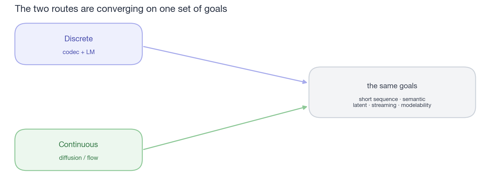
caption: “Two routes, one destination. Whether you start from discrete (codec + LM) or continuous (diffusion / flow), you end up solving the same set of problems: shorter sequences, a semantic latent, streaming, modelability. The surface ‘discrete vs continuous’ debate is really converging toward the middle.”

Step back and look at what the previous three chapters laid out, and you’ll find something easily obscured by the “discrete vs continuous” opposition narrative: the two directions are actually converging toward the same set of goals. No matter which end you start from, you end up solving the same three problems —

• How to make the representation sequence shorter: discrete here compresses the frame rate (Mimi 12.5 Hz, TADA 2–3 Hz), continuous here compresses both dimension and frame rate (VibeVoice 7.5 Hz) — the goal in both is to make the downstream LM’s context burden small enough to learn.
• How to make the representation more structured and more modelable: discrete relies on semantic distillation / hierarchical supervision, continuous relies on semantic anchoring (REPA / Dasheng / Ming-UniAudio) — both essentially inject semantic structure into the representation to make it friendly to the generative model.
• How to balance reconstruction quality and modelability: §3.5’s triangle, the two directions face the same triangle, just entering from different corners.

In other words, discrete and continuous are two coordinate systems of the same problem, not two opposing directions. Their tools (the two toolboxes of §2.5 and §3.2) are nearly mirror images, and the difficulties they have to solve are the same batch.

And — they need not replace each other; they can fully coexist and complement each other. The most ready-at-hand example is the staged coexistence of CosyVoice / Seed-TTS: the front segment’s discrete tokens do content planning (benefiting from LM infrastructure), and the back segment’s continuous flow does acoustic detail (eating generation quality). But coexistence isn’t limited to “staged” — a more radical possibility is using both representations on the same LM backbone simultaneously: letting the model both spit out discrete tokens (handling streaming, handling alignment with text) and spit out continuous vectors (handling high-fidelity generation), switching between the two heads by task. This road is still early, but it points to a much healthier future than “who replaces whom”: discrete and continuous aren’t an either-or that’s like fire and water, but two tools in one representation system, each handling a segment.

This is also why this chapter no longer fusses over “discrete or continuous” — the real controversy lies somewhere deeper.

4.2 What will the unified interface be — a deeper RVQ, or lighter continuous features?

After laying out so much, we’ve reached the place to render a judgment. First look at the current factual landscape.

On the understanding side, continuous features lead. On tasks like ASR, emotion recognition, and speaker verification that depend on “understanding” or “hearing detail clearly,” continuous SSL representations (typically WavLM) keep a sizable lead over all forms of discrete tokens — the gap is largest for pure acoustic codecs (EnCodec, DAC), next for semantic-distilled codecs (SpeechTokenizer, Mimi). In low-resource scenarios and complex acoustic scenarios the gap widens further.

On the generation side, discrete tokens started earlier and have a thicker ecosystem. All of the AR LM’s engineering dividends (KV cache, speculative decoding, in-context learning), the mature paradigm of zero-shot voice cloning (the VALL-E family), and the early complete systems of streaming real-time dialogue (Moshi) — all ran successfully on discrete tokens first. But note that real-time full-duplex “listen and speak at the same time” was once treated as discrete AR’s exclusive territory, and this monopoly has recently been broken by the continuous direction: Thinking Machines’ TML-Interaction-Small (2026)⁷⁴ uses dMel input + flow head output, interleaving 200ms micro-turns to listen and speak at the same time — a fully continuous full-duplex system with no discrete token whatsoever. So the more accurate statement isn’t “discrete is more mature,” but that discrete started early and the engineering debt still has to be slowly paid down by the continuous direction — and this gap is being closed quickly.

Here I have to add a judgment of our own, because it explains why more and more recent work is turning to continuous features for generative modeling (continuous autoregression) rather than discrete tokens — this turn is often read as “continuous finally won,” but I think the more accurate explanation is: the game the field is currently playing has changed, and this new game happens to be unfavorable to discrete.

Let me say it plainly. Discrete tokens’ true killer move was never the things they show off today, but one thing that hasn’t truly happened yet — like text, doing self-supervised pretraining on massive audio-only data. If the metaphor “audio as language” is to be cashed out, it depends on this: next-token pretraining, scaling laws, emergent abilities, the whole set of text-LLM dividends replicated onto audio. But the reality is that almost no one today does pure audio pretraining at text’s scale. The field’s true center of gravity is something else — the alignment of audio and text: either for understanding tasks (ASR, audio QA, audio-LLM), or for multimodal/real-time dialogue. The center of gravity is on alignment, not audio-only pre-training.

Once you see this clearly, that earlier empirical fact of “continuous leads for understanding” gains a structural explanation, not just the shallow “continuous features carry richer information”: in this game of alignment, discretization is pure loss, and its compensating advantage (pretraining scale) hasn’t been activated at all. Compress audio into discrete tokens, and what you discard is largely the fine-grained information that alignment and understanding need most; meanwhile, the “text-style large-scale pretraining” that should offset this loss hasn’t been done by anyone. The loss is fully laid out, the dividend fully idle — for continuous features to prevail in this setup is largely natural.

These two things each have an information-theoretic theorem backing them, not just intuition. “Discretization is pure loss” corresponds to the data processing inequality: any deterministic processing doesn’t increase information, \(I(X;\,\mathrm{quant}(Z)) \le I(X;Z)\) — quantization only loses, never adds. And “a pure-reconstruction latent isn’t friendly to understanding / alignment” corresponds to the information bottleneck (Tishby et al.): the optimal representation for downstream task Y is the minimal sufficient statistic that minimizes \(I(X;Z)\) while preserving \(I(Z;Y)\); but the reconstruction objective wants exactly the opposite — to maximize \(I(X;Z)\) (keep everything in order to recover the waveform). One is minimizing, one is maximizing, the directions twisted against each other. So “the reconstruction-optimal latent isn’t the downstream-optimal latent” isn’t an empirical observation, it’s that these two objectives, information-theoretically, simply don’t point at the same point.

So the continuous direction’s current upward trend, rather than being intrinsically stronger, is more that the field’s objective function happens to step right on discrete’s weakness and dodge discrete’s strength. This judgment has a slightly uncomfortable corollary: if one day pure audio large-scale pretraining truly becomes the mainline (compute, data, and motivation all in place), discrete’s idle ace might be reactivated and the situation might flip again. In other words, who prevails in discrete vs continuous essentially depends on what the field is optimizing — and that thing changes.

If this division of “understanding to continuous, generation to discrete” could be maintained often, they could coexist peacefully — each going its own way. But audio happens to have an unavoidable need forcing the two sides to merge: 4o-style real-time dialogue requires one model to listen and speak at the same time. Listening and speaking are coupled in physical time — listening while speaking, a latency budget of a few hundred milliseconds, bidirectional in parallel. The vision domain is also doing unified understanding + generation (Chameleon, Janus, Show-o, Emu3), but the driving force differs in intensity: vision’s unification is a nice-to-have of multimodal engineering, and understanding and generation in the product are usually asynchronous (upload an image, ask a question, generate an image — serial is fine); audio’s unification is a must-have of the product’s physical constraints — Chameleon doesn’t need to look-and-draw within 200ms, but 4o must listen-and-speak within 200ms.

So the question isn’t “will unification happen,” but: what will the unified interface look like? I see two directions that both have a real chance.

Direction one: a deeper, more structured RVQ codec — let discrete tokens carry both understanding and generation.

Three arguments for why it has a chance.

First, information capacity is actually enough. First, a rough calculation: continuous WavLM is 1024-dim float (≈ 32 kbits/frame of storage bit-width — not equal to effective information content, since neural features have a lot of redundancy, but the order of magnitude is usable for intuition); today’s discrete schemes — Discrete WavLM single-codebook k-means about 10 bits/frame, Mimi 8-layer RVQ ≈ 88 bits/frame — are respectively 3000× and 400× bit-width compression. Under this capacity configuration, losing to continuous isn’t a miscarriage of justice. And how much information do understanding tasks really need? Speech understanding doesn’t need all the sample detail of the waveform — 80-dim log-mel has long been the standard input of ASR / HuBERT / WavLM / Whisper, and classic ASR can run with 13–40-dim MFCC. The input end needs only on the order of a few kbits per frame to “understand.” Then 64-layer RVQ × 10 bits = 640 bits/frame, in the same order of magnitude as mel’s effective information content — total information isn’t the bottleneck. The reason no one today does the experiment of “64-layer RVQ + an understanding downstream that can consume a multi-codebook stream” is that RVQ codecs have always served generation (the more layers, the more it hurts AR unrolling), not that it’s infeasible in principle. “RVQ loses to continuous on understanding” is currently an empirical fact, not a mechanistic conclusion.

Second, the hierarchical structure naturally fits the dual-task division of labor. Understanding tasks read the first few layers (semantic layers), generation tasks use all layers (semantic + acoustic) — RVQ’s hierarchy lets the same token stream be consumed on demand. This property isn’t held by a single codebook nor by continuous features; it’s a structural dividend unique to RVQ.

Third, the current gap looks more like a paradigm artifact than a fundamental limit. In vision, early VQGAN multi-codebook was once thought to have “poor modeling performance,” until the downstream consumption mode was redesigned and it turned around. No one in audio has seriously done this redesign yet.

But direction one has a key premise, and it’s also the most easily overlooked trap: deepening the layers is far from enough; it must be paired with structural supervision. If you train a 64-layer RVQ with pure reconstruction loss alone, you get a codec with excellent reconstruction — and then it’s easy to assume “these tokens perfectly represent the audio.” But what the tokens store isn’t “the original information of the audio,” but “the information the decoder needs to recover the audio” — these two things aren’t the same. The decoder is a network with structure and inductive bias, able to fill in a great deal from priors (convolutional locality, periodic activation, etc.), so the tokens only need to carry the part “the prior can’t fill in” — a more entropy-dense, more entangled form. For a downstream LLM, these pure-reconstruction tokens may be even harder to read than feeding mel directly — the LLM doesn’t have those priors of the codec decoder, and it faces a string of “the decoder’s private language.” This is why the four paths of §2.3 (distillation / hybrid encoder / supervised / disentanglement) appeared in unison — they’re all doing the same thing: making the token’s structure friendly to the downstream LM, not just to the decoder. Tokens trained with pure reconstruction are “the decoder’s private language,” and only adding structural supervision turns them into “a public language the LLM can read too.”

So direction one’s full recipe is the joint design of three things: deep enough hierarchy + structural token supervision + a downstream model that can consume a multi-codebook stream. None can be missing, and no one today has done all three at once.

Direction two: lightweight, low-dimensional continuous features designed for modeling — bypass discretization and directly make the unified interface. §3 already discussed this road thoroughly, so I won’t re-expand here, just collect it into a judgment. On the understanding side, continuous is already the incumbent champion, one corner for free; on the generation side, continuous AR + flow head (§3.4) is maturing fast — VibeVoice⁷⁵ and DiTAR pushed up the unidirectional quality, and TML-Interaction even achieved full-duplex. And the key premise of making the unified interface — “continuous features must be specially designed for modelability” — is largely the same question answered by §3.3’s toolbox, §3.2’s semantic anchoring, and §3.5’s dimension triangle. DashengTokenizer⁷⁶, WavCube / LoSATok, and MingTok have already given prototypes of a continuous latent that can both understand and generate, so direction two is no longer just an idea. So its full recipe is also the joint design of three things: a semantically anchored low-dimensional latent + a mature continuous AR skeleton + a distribution head that can withstand streaming — the first two already have prototypes, and the last (the streaming stability of high-dimensional latents, §3.5) hasn’t been verified, which is the only hard bone direction two has left.

On the surface the two directions are a discrete-vs-continuous contest, but the requirement they place on representation design is actually the same one: the representation must be designed for downstream modeling — not just for reconstruction (the codec’s traditional goal) or just for recognition (SSL’s traditional goal). Direction one’s “structural supervision” and direction two’s “modelability design” are the same need expressed in two forms. This is the version that pushes Sander’s modelability dimension to the extreme: in the objective function of representation design, the downstream model’s consumption mode goes from an afterthought to a first-class citizen.

My own judgment: in the short term, direction two’s hybrid form (CosyVoice / Seed-TTS’s “single-layer semantic VQ + flow matching”) has already run successfully in products and has a first-mover advantage; in the medium term the two directions will evolve in parallel, and whoever first builds a complete system that’s “dual-optimal at understanding and generation” defines the next-generation standard. As for RVQ’s hierarchy itself — whichever direction prevails, I believe the property of “hierarchical/structured representation” won’t disappear: FACodec’s explicit factorize, SNAC’s multi-scale, even direction two’s hypothetical “continuous latent designed for modeling,” are all different incarnations of the hierarchical idea.

4.3 Audio’s fixed-grid constraint is more severe than vision’s

An important observation Sander makes in the original is the fixed-grid constraint — the vision latent treats every spatial position equally, wasting capacity. In one image, large swaths of background texture and the key foreground detail occupy equally many tokens, which is clearly not an optimal allocation of information.

This is more severe in audio but discussed less.

Audio’s redundancy is more uneven than an image’s.

• Speech has a lot of silence, pauses, sustained-consonant segments, stable-vowel segments — the information content of these positions is far below key moments like consonant burst points, vowel onsets, and prosody changes.
• Music has intro/outro, single-texture segments, long beats — the information density is likewise extremely uneven.
• But all of today’s mainstream codecs (EnCodec, DAC, Mimi, SoundStream) are constant frame rate (50 / 75 / 12.5 Hz), producing equally many tokens whether speaking or silent. This is the core symptom of the fixed-grid constraint in audio.

Why “constant frame rate” loses in principle, rate-distortion theory puts it bluntly: to encode a source, the optimal strategy is to make the local bitrate match the local entropy rate — give more bits where there’s more information, fewer where there’s less. And speech is a highly non-stationary source, with the instantaneous entropy rate near 0 in silence and spiking abruptly at the instant of a plosive or vowel onset. Encoding it with a constant frame rate is like burning money at high bitrate on silence while undersupplying bits at the high-entropy instant — an obviously suboptimal point on the rate-distortion curve. So variable-length / content-adaptive tokenization “should” win not as engineering flair, but because it aligns the bitrate to the entropy rate, approaching rate-distortion optimality — which is exactly the old lesson entropy coding (the arithmetic-coding class) has preached for decades, only this time moved onto the frame rate of a neural codec.

The vision domain is already rebelling. Over the past two years, a batch of content-adaptive work has appeared in vision tokenization:

• TiTok (Yu et al., 2024)⁷⁷ — uses a transformer to compress an image into a variable number of tokens (32 or 64), proving the fixed grid isn’t necessary.
• FlexTok (Bachmann et al., 2025)⁷⁸ — the number of latent tokens is dynamically adjusted at inference time by content.
• ElasticTok, CAT: Content-Adaptive Image Tokenization, TokenSet, etc. — attacking the fixed-grid assumption from different angles.

Corresponding work is starting to appear in the audio domain, but the scale gap relative to the vision community is still large. What can be brought out for comparison:

• Sander’s own 2021 Variable-rate discrete representation learning⁷⁹ — an early but long-lonely work.
• SoundStream’s quantizer dropout — only “soft variable-length” (one model working at different bitrates), not true content adaptivity.
• SNAC’s MSRVQ — different RVQ layers at different frame rates, but within each layer still constant.
• ALMTokenizer (Yang et al., ICML 2025)⁴⁵ — uses query-based quantization to achieve a low-bitrate semantic-rich codec, the audio counterpart of TiTok’s query-based direction: replacing the fixed 1D time grid with learnable queries, relating the number of tokens to the content.
• TADA (Dang et al., Hume AI, 2026)⁸⁰ — a more radical approach: aligns audio tokens 1-to-1 to the LLM’s text tokens via CTC + Viterbi forced alignment. This way the production of audio tokens is no longer “one per X milliseconds,” but “one per text token” — fast speech produces more tokens, slow speech/silence produces fewer. The result is a 2-3 FPS content-adaptive frame rate, an order of magnitude lower than Mimi’s 12.5 Hz. This is the most extreme variable-length audio codec to date.
• FlexiCodec (Li et al., ICLR 2026)⁸¹ — does dynamic frame rate directly inside the codec: using frozen ASR features as a “semantic ruler,” it merges adjacent frames whose inter-frame cosine similarity exceeds a threshold into one frame — merging more where information is sparse (silence, steady-state vowels) and keeping more where it’s dense, with the threshold adjustable at inference, and the average frame rate landing in 3–12.5 Hz. The merging step likewise goes query-based⁴⁵: stuffing one query token into each segment to summarize the original frames within the segment, the only difference being that the number of queries is dynamically determined by similarity. Its virtue is that it doesn’t rely on a text anchor — purely on inter-frame semantic similarity, so in principle it holds for music and general audio too, which is exactly where TADA’s text-aligned direction can’t reach. But the boundary is clear too: it uses full-sequence ASR features, an offline design, and doesn’t solve streaming; and before decoding it uses a frame-unmerging module to re-expand the variable-length sequence back to a fixed-length 12.5 Hz before feeding downstream — dynamic inside the codec, but a fixed-length stream to the outside, with “letting downstream directly consume dynamic-rate tokens” listed by the paper as future work.
• SAME (Parker et al., Stability AI, 2026)⁶⁸ — ports the same set of query-based compression onto the continuous side: it’s a continuous autoencoder for music / general audio (44.1 kHz stereo, 4096× compression, d=256, the bottleneck being soft-normalisation rather than a strict VAE), with resampling done by a Transformer Resampling Block — appending a learnable query embedding after each segment, passing it through a transformer to let it attend to the original frames within the segment, then extracting it as the compression result. This is the same kernel as ALMTokenizer, except ALMTokenizer goes discrete + variable-rate and SAME goes continuous + fixed stride. So strictly speaking SAME itself doesn’t rebel against the fixed-grid constraint — its query count is sliced out at fixed length and the frame rate is constant; its significance is in showing that query-based compression is no longer a discrete-codec patent — continuous music autoencoders use it too. Swapping the fixed stride of SAME-class continuous autoencoders for FlexiCodec-style content-adaptive merging is an obvious but as-yet-unwalked next step.
• Some streaming codecs explore VAD-based skip or silence-aware down-sampling, but there’s no mainstream scheme.

Even adding these works, the audio community’s exploration of variable-length tokenization still lags vision’s — on the vision side, TiTok / FlexTok / ElasticTok / CAT / TokenSet have already formed a research direction with volume, while on the audio side ALMTokenizer, TADA, and FlexiCodec are still relatively scattered explorations, not yet forming a sub-field in dialogue with one another.

Regarding the “conflict” between streaming + variable-rate, I need to correct my initial judgment: these two things aren’t largely irreconcilable. TADA gives an interesting solution — using a text-token clock to replace the audio-time clock. Audio tokens are no longer produced uniformly by physical time, but advance forward together with text tokens at a synchronized rhythm; it’s both streaming (a pair of text+audio tokens produced each time) and variable-rate (the same number of text tokens can correspond to different lengths of audio). This is a clever design — shifting the burden of “variable-length” onto the text end, letting the audio end keep its rhythm stable.

These several works each gnaw off a part of the difficulty: TADA proves “with a text anchor, variable-length and streaming can be had together” (using a text-token clock to replace the audio-time clock, producing a pair of text+audio tokens each time, both streaming and variable-length); FlexiCodec proves “without relying on text, content-adaptive frame rate can be made from inter-frame semantic similarity” — covering the music / general audio that TADA can’t reach.

So the full version of this Observation is this: audio’s fixed-grid constraint is more severe than vision’s (the signal’s own redundancy distribution is more uneven), but the good news is that the few puzzle pieces rebelling against it have appeared one after another in the past year or two. What truly hasn’t been assembled is doing three things at once: no text anchor, content-adaptive, and causal streaming — FlexiCodec takes the first two, but it’s offline and non-streaming, while TADA is streaming but relies on text. A deeper difficulty is still downstream: having an LM natively consume a variable-length stream whose “tokens per second floats with content” (rather than first padding or unmerging into fixed length), something almost no one touches — even the most cutting-edge FlexiCodec is dynamic inside the codec and unmerges back to fixed length before decoding to bypass downstream, and even it lists “downstream directly eating the variable-length stream” as future work. The vision community has a batch of star works like TiTok / FlexTok pushing variable-length tokenization into a mainstream topic, while audio is just getting started — whoever first assembles the four things “general audio + streaming + content-adaptive + downstream-consumable” will occupy a key position in the infrastructure of the next generation of audio LMs.

4.4 Adding streaming to Sander’s rate-distortion-modelability triangle

One of the most influential concepts in Sander’s original is the rate-distortion-modelability triangle — any latent design makes a trade-off among these three dimensions:

• Rate: how many bits the latent occupies. The harder it’s compressed, the smaller the downstream modeling burden.
• Distortion: how much the signal is distorted when reconstructed back from the latent. The less distortion, the higher the quality.
• Modelability: how friendly the latent is to the downstream generative model. The more structural, the better the modelability.

A few specificities of audio require adjusting this triangle:

1. The distortion dimension is harder to quantify than in vision — there’s no recognized differentiable perceptual loss like LPIPS, and all distortion measures (PESQ, UTMOS, ViSQOL) have biases. §1.1 discussed this. The practical implication is: codec designers are “tuning blind” on the distortion dimension, relying only on indirect approximations like the multi-discriminator. This amplifies the “philosophical divergence” §2.1 discussed — EnCodec and DAC, under the same nominal “distortion,” are actually optimizing different things.

2. The modelability dimension is strongly coupled with “sequence length” — even compressed to 12.5 Hz, the audio latent sequence of a 30-second audio is still hundreds to a thousand-plus tokens. This is a challenge for attention, and for streaming too. So “modelability” in audio is not only “whether tokens are well-structured between each other,” but also implicitly “whether the token stream is short enough to be processed efficiently by an LM.”

3. A new dimension must be added — Streaming / latency. Streaming isn’t unique to audio (it exists in video streaming, robot interaction, and video generation too), but audio’s real-time dialogue turns it from an engineering preference into a hard product constraint — you must listen and speak within a few hundred milliseconds, a latency level vision applications rarely face. The streaming dimension directly shapes multiple details of representation design:

• Causal convolution vs non-causal — determines whether the codec can stream.
• AR vs non-AR modeling — determines whether downstream can stream.
• Variable-rate vs fixed-rate — streaming compatibility is largely different.

So Sander’s triangle, in audio, should be extended into a tetrahedron — adding streaming, the fourth dimension that doesn’t exist in vision and was forcibly handled by the product form.

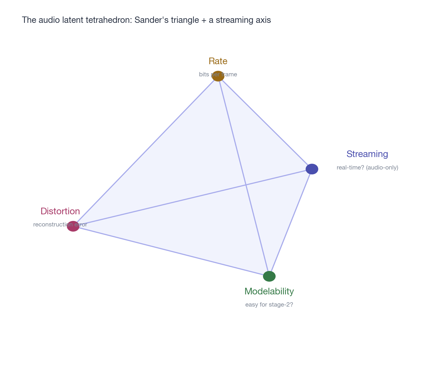
caption: “Rate, Distortion, and Modelability are Sander’s original triangle, and Streaming is audio’s unique fourth dimension. Any audio latent design is a trade-off point inside this tetrahedron — and the two ‘real controversies’ from the introduction are largely two edges of the tetrahedron: sequence length vs per-frame capacity is the Rate–Modelability edge, streaming vs offline is the Streaming–Distortion edge.”

With the tetrahedron explained, the two “real controversies” from the introduction each fall into place: sequence length vs per-frame capacity is a Rate–Modelability contest (Mimi’s low frame rate, high capacity vs WavTokenizer’s high frame rate, single codebook, with neither crushing the other); streaming vs offline is a Streaming–Distortion contest (discrete AR is streaming-friendly but per-frame capacity is limited, continuous NAR is high quality but hard to stream). Neither controversy is “continuous vs discrete,” but a matter of which corner of the tetrahedron to choose.

But there’s one more thing falling outside the tetrahedron — it asks not “how well the representation models itself,” but “how well the representation grafts onto an existing text LLM”: who can train more easily together with a pretrained text LLM? In the multimodal era this may be the most realistic decider, because no matter how elegant a representation is, if it can’t reuse a text LLM’s weights and training infrastructure, the deployment cost is an order of magnitude higher. There’s no simple winner on this dimension: discrete’s interface is naturally compatible (expand the vocabulary, reuse the embedding, cross-entropy unchanged), but compatible doesn’t equal efficient — the granularity of audio and text tokens differs greatly, and the codebook geometry isn’t aligned with the text embedding (LLM-Codec initializing the codebook is largely forcibly fixing this); the continuous side has heterogeneous losses (the flow head isn’t softmax, and the ratio and gradient balance of mixed training are real problems), but the batch of semantically anchored continuous latents may instead align more naturally with the LLM semantic space — after all, they grew out of the features of understanding models to begin with.

Putting the tetrahedron together with this out-of-system axis, the whole article’s judgment is one sentence: what truly decides the future of audio generation isn’t “continuous or discrete,” but how to trade off along these few underlying dimensions. The two directions will continue to lean toward the middle and borrow from each other, ultimately most likely fusing into a kind of hybrid representation “from which you can’t tell which direction it came from” — and what shapes the infrastructure form of the next decade is these trade-offs themselves.

5. Closing: open problems

Having finished telling the latent-design history of a field, what’s left for the future is a series of undecided questions. This section lists four directions I think worth watching over the next 1-3 years — the last one will shake the very premise of this whole article.

Will audio converge to a single unified latent?

Vision once walked to such a “moment of convergence”; it’s worth first seeing clearly what it actually was, lest we misattribute the credit. Convergence didn’t happen at the moment VQGAN was released in 2021, but when Stable Diffusion pushed the latent diffusion template into the de facto standard in 2022 — and interestingly, the unified carrier wasn’t VQGAN’s discrete tokens (the discrete AR direction of DALL-E 1 / Parti / MUSE actually didn’t become mainstream), but the continuous KL-VAE “trained by the VQGAN recipe but with quantization removed.” What VQGAN truly left for posterity wasn’t that codebook, but its training recipe: reconstruction loss + LPIPS + patch adversarial — this set of recipes moved into SD’s VAE and became the latent foundation of nearly all subsequent image/video generation models. So the precise meaning of vision’s “moment of convergence” is: a certain learned latent’s training recipe + a killer downstream application made the whole field converge onto the same latent template within a year or two.

Will audio have such a moment?

In the short term I don’t quite believe it — both the discrete and continuous directions (§2, §3) are still evolving fast, and within each direction there are multiple sub-schools (compression-school, semantic-school, disentanglement-school, single-codebook-school, etc.), none of which has yet seen the combination of “training recipe reused field-wide + a killer application pulling convergence.” EnCodec, DAC, and Mimi all have the potential to become templates, but each has an obvious design-philosophy bent, and all are a step away from a “general latent.”

What may appear in the medium term isn’t a single codec, but some kind of API-compatible standardized interface — waveform in, multi-codebook RVQ stream out, first layer phonetic-aligned. This way the downstream LM / diffusion needn’t care which specific codec it is. This kind of “interface standardization” happened in vision (after SDXL, VAE-KL 8× became the de facto standard), and there’s reason to believe a similar event will happen in audio — as for whether this interface is more likely a deeper RVQ or lighter continuous features, §4.2 already weighed the odds of the two directions.

End-to-end is harder in audio than in vision

The vision community walked the road of VAE → VQGAN → latent diffusion very smoothly, each generation a kind of clear end-to-end evolution. In audio, end-to-end has never truly prevailed — TTS to this day is still the multi-stage splice of text → semantic token → acoustic feature → vocoder. §1 explained the reason: the phase paradox + the lack of a differentiable perceptual loss + the long-sequence constraint make “one model from start to finish” especially hard in engineering.

The concrete manifestation of this is that neural codecs have been around for five years, yet the codec is almost never end-to-end co-trained into the downstream generative model — VALL-E, Moshi, and CosyVoice all train the codec first and freeze it, then train the LM on top. This differs from the vision practice in SDXL of “the latent VAE and diffusion co-trained.” If in the coming years someone gets audio codec + downstream truly co-training to run, the dichotomy of discrete and continuous will blur further; if it can’t run, the two-stage paradigm will persist long-term as audio’s “path-dependent reality.”

The place of the audio latent in the multimodal era

After “unified architectures” like GPT-4o appeared, audio is no longer an independent research domain — it must share a transformer backbone with text / image / video. This places new hard constraints on audio latent design:

• The audio latent will be pushed toward a token-like interface — when crossing modalities, the transformer backbone needs to be able to consume it efficiently. This can be explicit discrete tokens, or low-frame-rate continuous embeddings connected via a projector / resampler; discretization is the most direct scheme to reuse the LLM’s next-token training, KV cache, and in-context learning, but it isn’t the only choice.
• The “speaking rate” of audio tokens must be coordinated with the speaking rate of text / image tokens — TADA’s text-aligned tokenization is largely a direct response to this.
• Cross-modal in-context learning requires audio tokens to carry structurally strong information, not the decoder’s private language — which is the “structural token supervision” repeatedly discussed earlier.

So the multimodal era isn’t simply stuffing audio into a multimodal transformer — it will in turn reshape the priorities of audio latent design. It’s not that audio evolves at its own pace and is finally absorbed by multimodality, but that multimodality’s needs push back on the audio latent, accelerating its evolution in a particular direction.

Will the audio encoder / codec simply disappear?

This last question shakes the premise of the whole article. This blog post assumes from start to finish that audio generation needs a latent intermediate layer — but two recent directions are probing “can we do without it?”: for understanding, multimodal models like Gemma 4 feed audio directly into the LLM; on the generation side, a batch of work (such as WaveTTS) returns to directly modeling the waveform. If both hold, then are the audio encoder and codec ultimately superfluous?

The most radical step for understanding is doing away with even the encoder. Gemma 4’s official statement⁸² is “remove the audio encoder largely, directly projecting the raw audio signal into the same dimensional space as text tokens” (consistent with its vision direction, both modalities encoder-free). No pretrained encoder, no intermediate features — raw audio passes through a projection layer to become token embeddings, and everything else is left to the shared transformer backbone.

This looks like “the encoder has mostly disappeared,” but the more accurate statement is that the function of encoding hasn’t disappeared, it’s just gone from an independent reusable module to being thoroughly dispersed into the shared backbone. Two details show it didn’t really disappear: first, the task of compressing high-entropy waveform into low-entropy semantics still has to be done by someone, and now it’s certain layers of the backbone doing it implicitly (that mel-80-dim argument still holds — understanding doesn’t need sample detail); second, and harder — raw audio is twenty-thousand-plus samples per second, and there can’t be twenty thousand tokens per second, so that “projection layer” still needs to map a block of samples to one token, and this “block→token” is itself frame-rate reduction, just done in an inconspicuous new place. The name “encoder” is gone, but the two things the encoder did — abstraction and rate reduction — neither disappears.

This is actually a rehearsal of the scaling-oriented view for understanding: rather than handcrafting an encoder, let a big-enough model + enough compute learn to encode itself. So the true trend for understanding isn’t “whether the encoder exists,” but “whether encoding should be made an independent module” — the value of an independent module is reusability, cross-task transfer, and separate optimizability, while the value of end-to-end absorption is not being stuck by human-designed inductive bias, letting scaling speak for itself.

The generation side’s “directly modeling the waveform” is the other side of the same scaling-oriented view — and it isn’t new. WaveNet (2016) and waveform diffusion (WaveGrad / DiffWave, 2020) both tried end-to-end waveform generation, and §3.1 explained why they lost to latents: the waveform is too long, sampling too slow. Now it’s making a comeback (the WaveTTS class), relying not on a new idea but on compute and architectural efficiency — leaner attention, better parallelism, turning “directly processing tens of thousands of samples” from infeasible to barely feasible. So the two ends are actually the same problem: when compute is sufficient, will the motive of “lossy compression / explicit encoding done to make downstream well-modelable” gradually fail, letting the model get closer and closer to the raw signal?

My judgment: the function of encoding won’t disappear, but it may no longer be an independent module; and streaming will limit this trend. In the short term, pure-compression codecs (the kind designed for transmission) may indeed give way — with enough compute, compression ratio is no longer a hard constraint, and the understanding side’s independent encoder may also be absorbed into the big model the way Gemma is. But the function of “tidying the signal into a well-modelable form” won’t disappear because of compute growth; on the contrary, as models grow larger and contexts grow longer, it becomes more important. More crucially, audio has that hard constraint vision doesn’t: listen-and-speak requires a compact representation. A real-time dialogue system can’t throughput tens of thousands of samples per frame — neither latency nor compute allows it. As long as streaming is audio’s core product form, compressing the signal into a low-frame-rate representation has an irreplaceable reason — whether this compression is done by an independent codec or quietly done by some layers inside the model.

Put back into the tetrahedron, this is largely a set of dynamic tension: the scaling-oriented view keeps weakening the importance of the Rate dimension (with enough compute you don’t care how hard it’s compressed), but the Streaming dimension keeps it important (real-time always needs compactness). So the most likely future isn’t “the latent disappears,” but offline high-quality generation increasingly daring to get close to the raw signal, while real-time interactive generation continues to rely on a compact latent — this line and the earlier division of “discrete handles streaming, continuous handles quality” are actually the same crack projected onto a different dimension.

Acknowledgments

Special thanks to Sander Dieleman’s Generative modelling in latent space. This post borrows its high-level framing and discusses the same question from the audio side.

The progress of this field over the past five years comes from the entire audio codec / audio LM community. Due to space limits, I couldn’t cite every relevant work, and omissions are inevitable — but this article is essentially a distillation standing on top of all of these works, and I want to thank all the papers that pushed this field forward.

The observations in this post represent my current understanding, and some of them may be incomplete or wrong. I very much welcome you to come discuss, ask questions, or directly point out where I got it wrong — find me on X (Twitter) at @dcyang98, by email at dcyang@se.cuhk.edu.hk, or on GitHub at @yangdongchao.

References